I am currently a PhD student at the Chemical and Materials Engineering Department of the University of Alberta. My research interests are in process control (mainly statistical), machine learning, and modelling and simulation of chemical processes. I am also interested in software, application and web development.

Previously, I completed my masters at the Process Engineering Department of Stellenbosch University. My research interests are in process control (mainly statistical), machine learning, and modelling and simulation of chemical processes. I am also interested in software and web development.

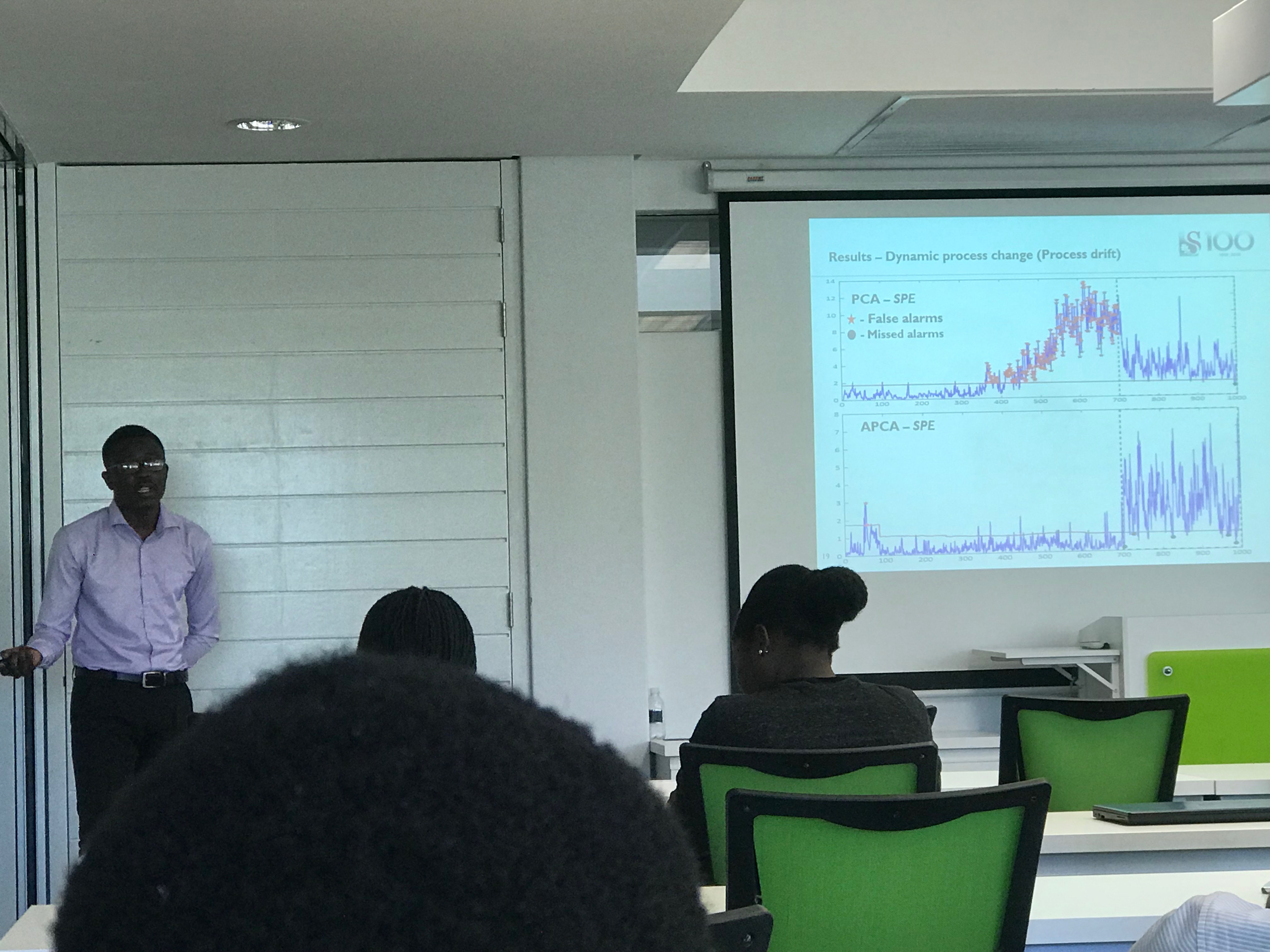
My master's work was on adaptive process monitoring with data-driven approaches, in which a novel monitoring approach that caters for slow and sudden process changes was developed. The work was funded by Sasol and The Center for Artificial Intelligence Research, South Africa, with notable contributions by the people listed below.

Dr. Lidia Auret

Data Science and Process Manager

Stone Three Digital

South Africa

Dr. Steve Kroon

Senior Lecturer

Department of Computer Science

Stellenbosch University

Dr. Roelof Coetzer

Senior Manager

Industrial Statistics

Sasol Group Technology

Dr. John McCoy

Data Scientist

Stone Three Digital

South Africa

PhD Process Control, University of Alberta (2020 - Present)

M.Eng. Extractive Metallurgical Engineering, Stellenbosch University (2017 - 2019)

B.Sc. Petrochemical Engineering, Kwame Nkrumah University of Science and Technology (2012 - 2016)

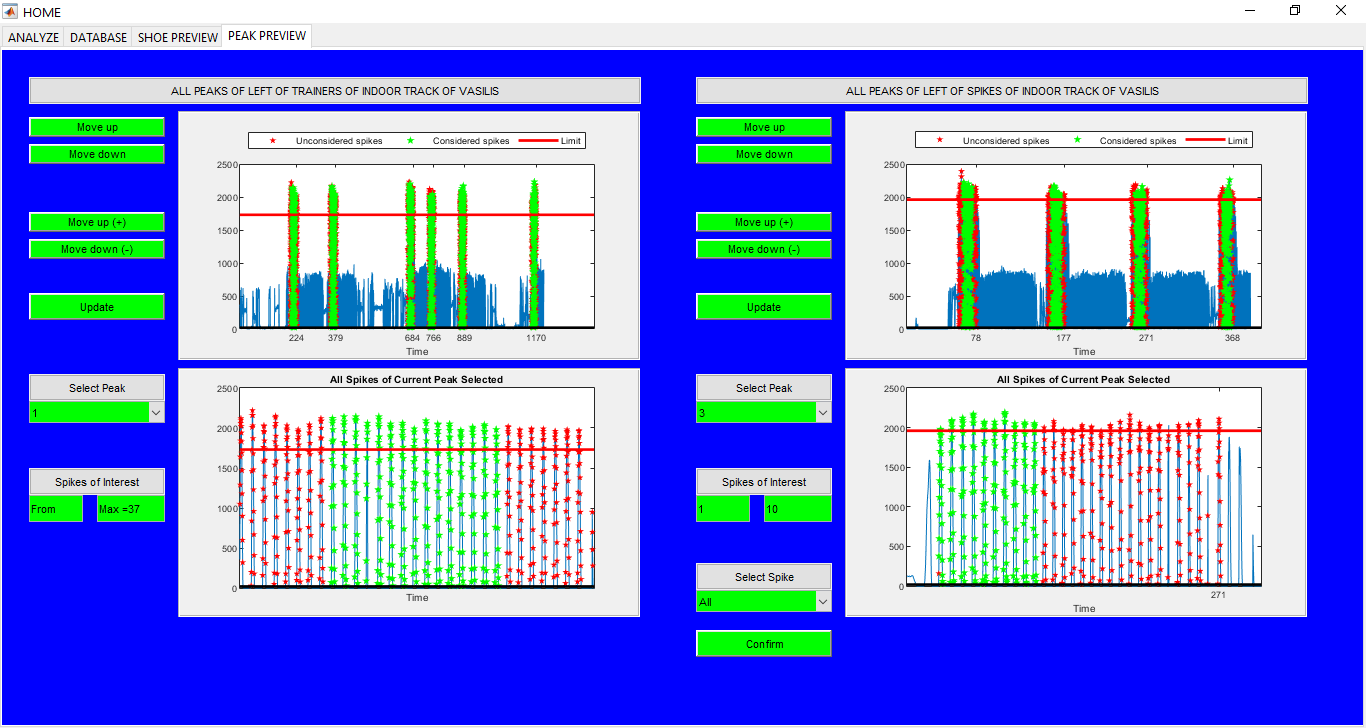
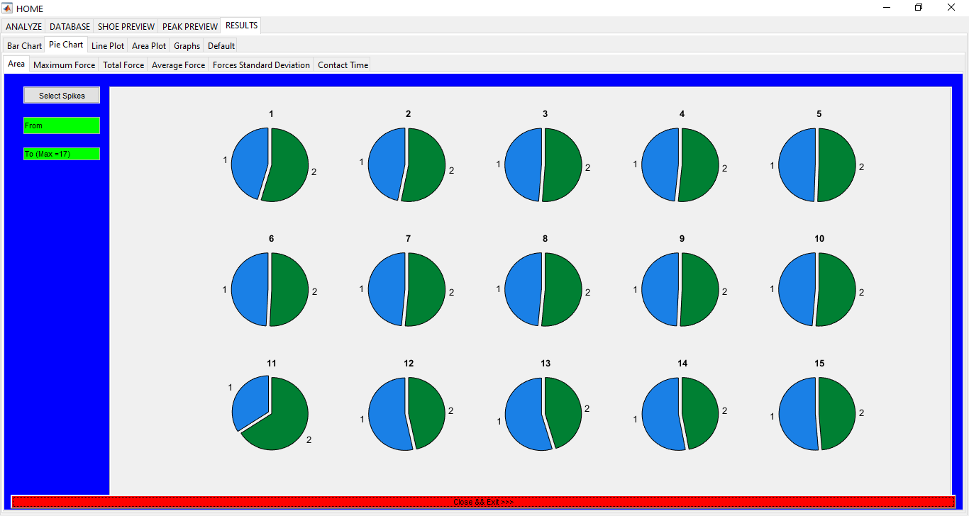
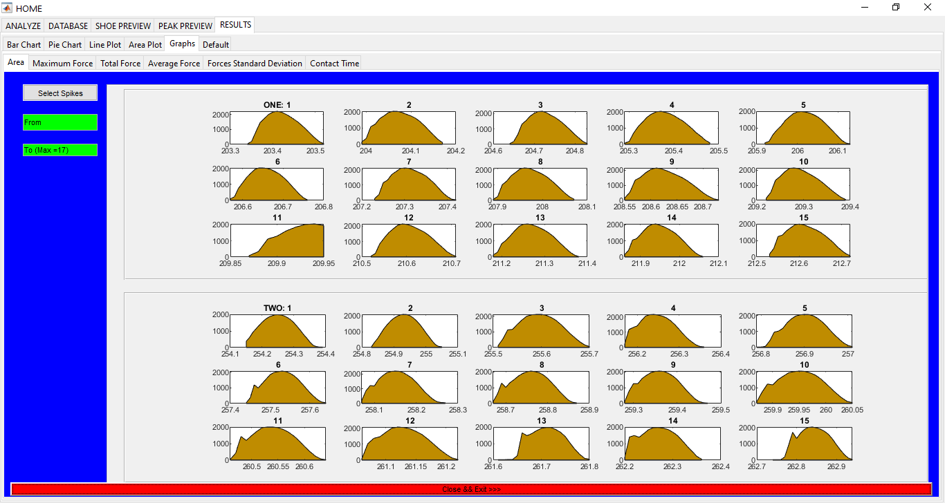
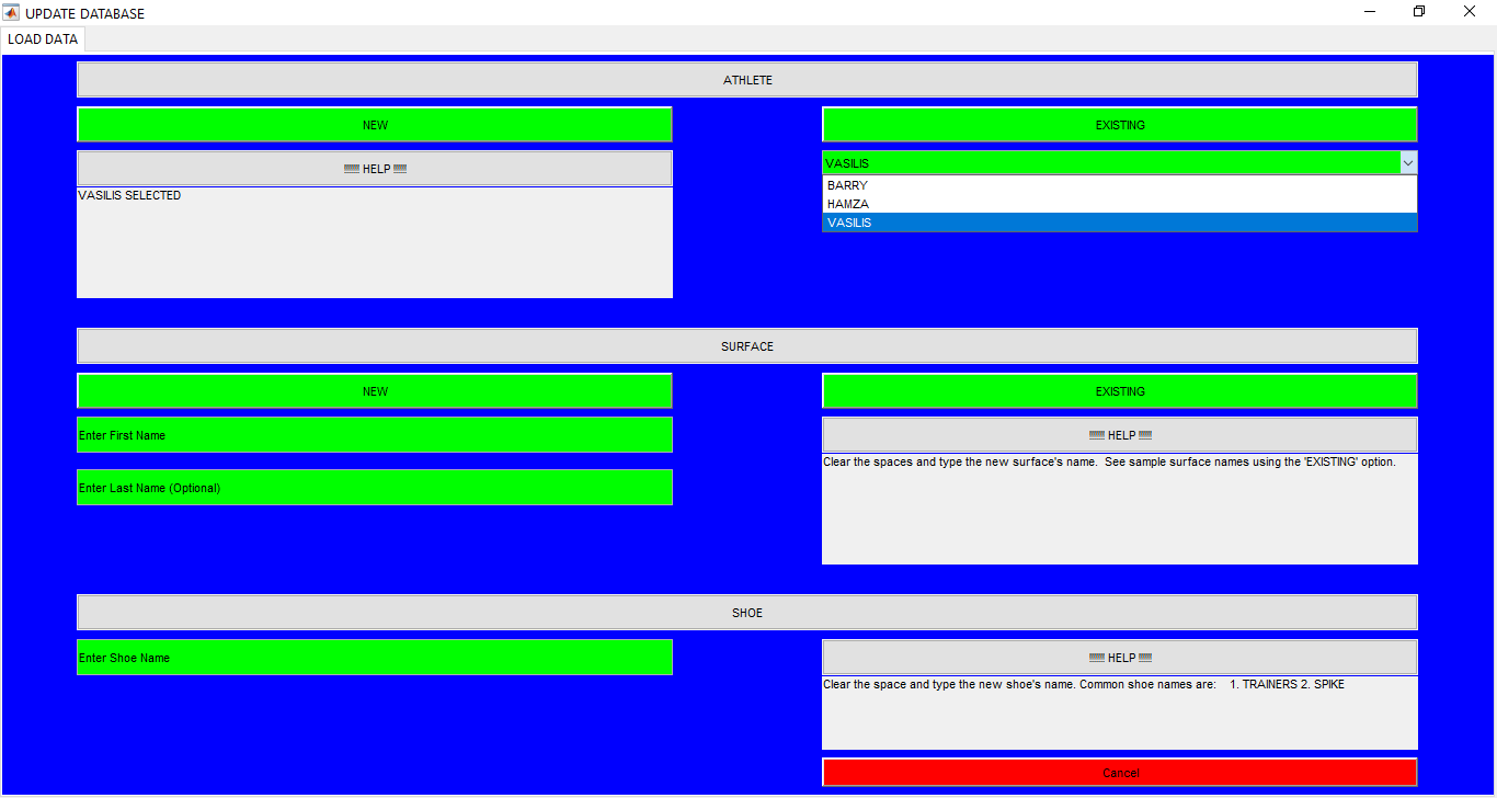
Sports Data Analytics Toolbox

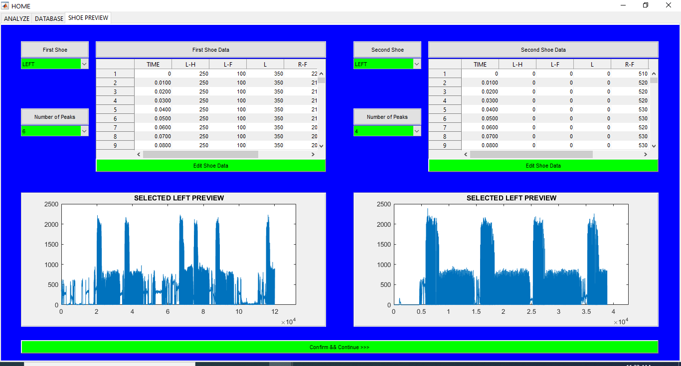
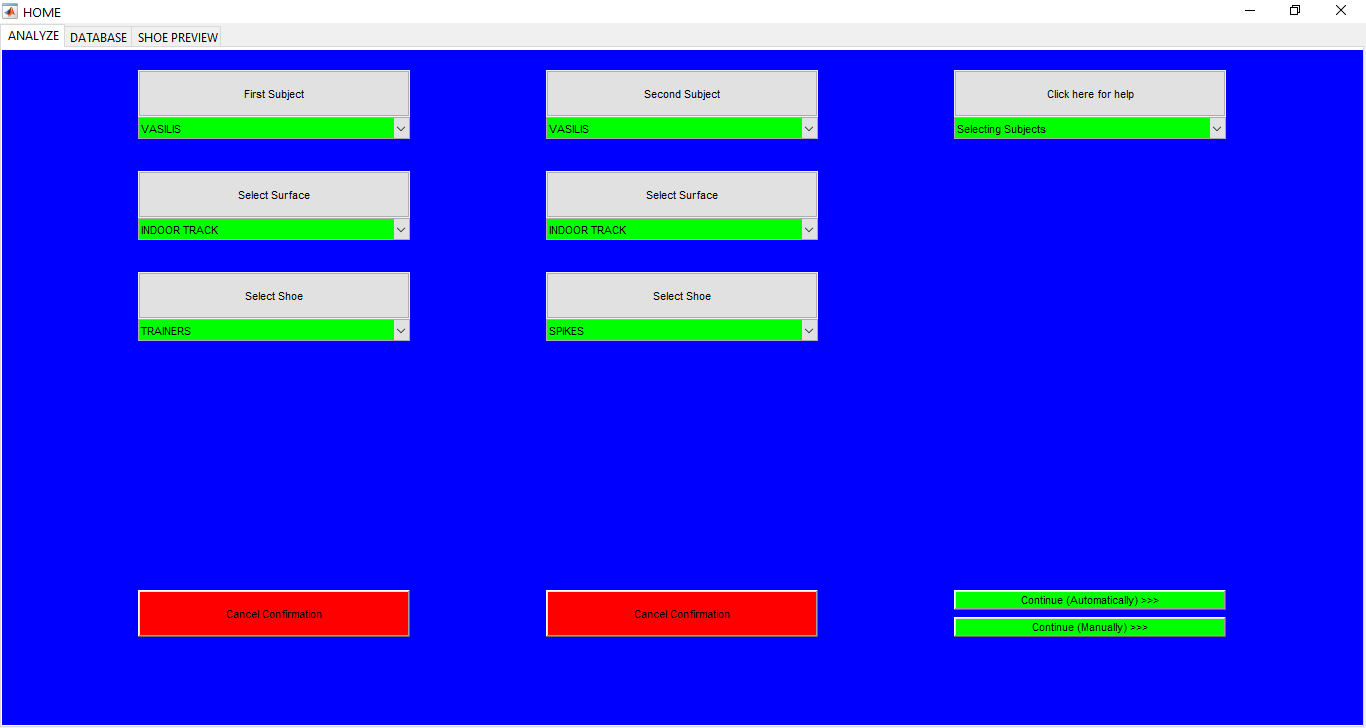
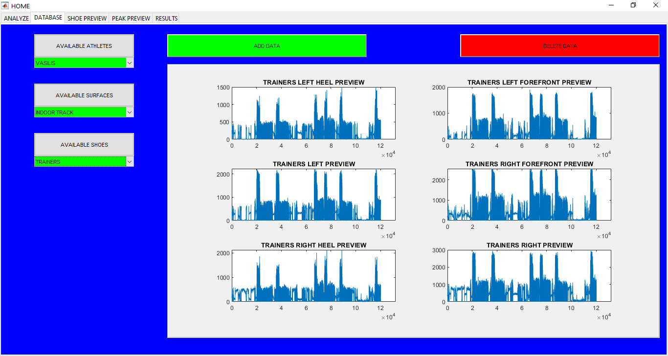
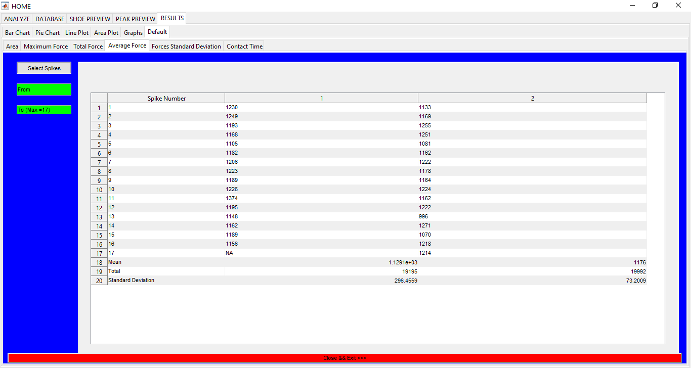
An App for sports data analytics for different subjects running in different shoes and on different surfaces. Database for all the shoes, surfaces, and the subjects is kept as well. ** UNLESS UNDER SPECIAL CIRCUMSTANCES, THIS APP IS NOT AVAILABLE FOR DOWNLOAD **

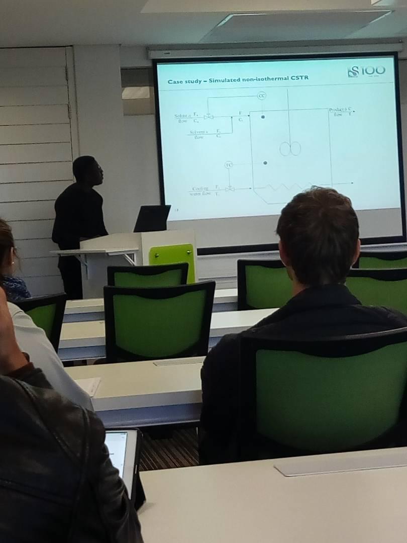
Non-Isothermal Continuous Stirred Tank Reactor (CSTR) Simulator

This work builds a Simulink model and a MATLAB program that uses graphical user interfaces (GUI) for simulating the Non-isothermal CSTR which was first developed by Yoon and MacGregor (2001) in fault detection. The model incorporates different works of the non-isothermal CSTR into a combined model that simulates a unimodal/multimodal operation data and different process faults as well as closed/open loop operation.

The non-isothermal continuous stirred tank reactor (CSTR) model is a popular model used by several authors (Choi et al., 2005; Alcala and Qin, 2010; Jeng, 2010; Mnassri, El Adel and Ouladsine, 2015; Mansouri et al., 2016) in data generation for fault detection, fault diagnosis, and other relevant purposes. Although it’s mentioned in the above-mentioned works, there is no readily available model for the simulator. Also, the different works (mentioned earlier) model different fault scenarios for the specific purposes without a generic simulator created.

Software requirements

The Simulink model is built using MATLAB R2017b version, therefore, MATLAB R2017b is required at least.

References

Alcala, C.F. and Qin, S.J., 2010. Reconstruction-based contribution for process monitoring with kernel principal component analysis. Industrial & Engineering Chemistry Research, 49(17), pp.7849-7857.

Jeng, J.C., 2010. Adaptive process monitoring using efficient recursive PCA and moving window PCA algorithms. Journal of the Taiwan Institute of Chemical Engineers, 41(4), pp.475-481.

Mansouri, M., Nounou, M., Nounou, H. and Karim, N., 2016. Kernel PCA-based GLRT for nonlinear fault detection of chemical processes. Journal of Loss Prevention in the Process Industries, 40, pp.334-347.

Mnassri, B. and Ouladsine, M., 2015. Reconstruction-based contribution approaches for improved fault diagnosis using principal component analysis. Journal of Process Control, 33, pp.60-76.

Yoon, S. and MacGregor, J.F., 2001. Fault diagnosis with multivariate statistical models part I: using steady state fault signatures. Journal of Process Control, 11(4), pp.387-400.

The CSTR process as shown in Figure 1.1 is a non-isothermal system with a single reactor tank. The reactor takes an input of premixed reactants (solute a and solvent s) and produces the product b. The reaction rate is a first order reaction based on the assumptions that there is perfect mixing; physical properties remain constant and there is negligible shaft work. The process is an exothermic one with a coolant maintaining the desired temperature. The reaction rate r is presented in Equation 1.1.

$r = k_oe^{-E/RT}C$

1.1

Here, k_o is the pre-exponential kinetic constant; E is the activation energy for the reaction; R is the ideal gas constant; C is the concentration and T is the temperature.

The behaviour of the dynamic process is described by the mass balance of the reactants , is shown in Equation 1.2, and the total energy balance as shown in Equation 1.3.

$\frac{dC}{dt}=\frac{F}{V}(C_i-C)r$

1.2

$\frac{dT}{dt} = \frac{F}{V}(T_i-T)-\frac{q(F_c)^{(b+1)}}{V\rho c_p(F_c + a(F_c)^b/2\rho_cc_{pc})}-(T_i-T_c)-(\Delta H_r)Vr$

1.3

Here, V is the volume of reaction mixture in the tank; F and Fc are the flow rates of the inlet reaction mixture and the coolant respectively and ρ and ρ_c are the densities of the inlet reaction mixture and the coolant respectively. The heat of reaction is denoted by ΔH_r. T_i and T are respectively the reactor inlet temperature and outlet temperature. The constants q and b are constants of the empirical relationship UA = qF_c^b, that relates the heat transfer coefficient UA to the coolant flow rate. Parameters c_p and c_pc are respectively the specific heat capacities of the reaction mixture and the coolant.

The concentration of the inlet reaction mixture C_i is given as an average of the solvent s and reactant a concentrations:

$C_i=\frac{(F_a C_a+ F_sC_s)}{(F_a+F_s )}$

1.4

Here, F_a and F_s are respectively the flowrates of reactant a and solvent s. C_s is the concentration of solvent s. F_a and F_sintuitively sum up to F.

The measured variables are the input variables F_a, F_s, F_c, C_a, C_s, T_c, T_i and the process output variables process T and C. For a closed loop process, the temperature of the reactor T is controlled by manipulating the coolant flowrate F_c. The concentration is also controlled by manipulating the flowrate of reactant a F_a.

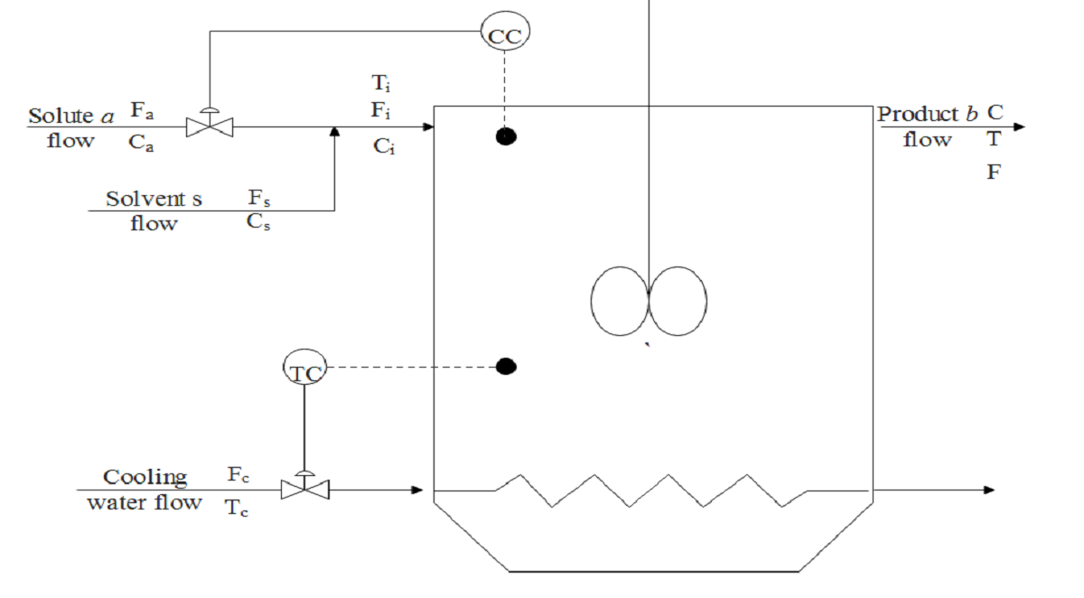
Figure 1.1: Non-isothermal CSTR flow diagram with concentration controller (CC) and temperature controller (TC).

The primary CSTR model is built using the material and energy balances provided in Equations 1.2 and 1.3. The relevant model parameters and modeling of process faults and multimodal operation and incorporated other process changes are presented in the subsequent sub-sections.

Parameters Modeling

The Simulink model uses simulation parameters and simulation conditions adopted from Yoon and MacGregor (2001). The descriptions and values of the relevant parameters and initial conditions are respectively presented in Table 1.1 and Table 1.2.

Table 1.1: Summary of reactor parameters.

Notation	Parameter	Value	Unit
V	Reaction mixture volume	1	m³
ρ	Density of reaction mixture	10⁶	g/m³
ρ_c	Density of coolant	10⁶	g/m³
c_p	Specific heat capacity of the reaction mixture	1	cal/(gK)
c_pc	Specific heat capacity of the coolant	1	cal/(gK)
ΔH_r	Heat of reaction	-1.3 × 10⁷	cal/(gKmol)
k_o	Pre-exponential kinetic constant	10¹⁰	min^-1
E/R	Activation energy/ideal gas constant	8330	K
q	inner film heat transfer coefficient	-1.678 × 10⁶	cal/minK
b	Empirical relationship of heat transfer and coolant flowrate constant	0.5

Table 1.2: Summary of reactor initial conditions.

Notation	Parameter	Value	Unit
F_s	Flowrate of solvent	15	m³/min
T_i	Reactor feed inlet temperature	370	K
T_c	Coolant temperature	365	K
C_s	Concentration of solvent	0.3	kmol/m³
C_a	Concentration of reactant	19.1	kmol/m³
F_c	Flowrate of coolant	15	m³/min
T	Temperature of reactor	368.25	K
F_a	Flowrate of the reactant	0.1	m³/min
C	Concentration of reactor	0.8	kmol/m³

A closed-loop simulation employs a PI control system with the controller parameters adopted from Yoon & MacGregor (2001) as shown in Table 1.3.

Table 1.3: Summary of parameters of the PI controllers.

Notation	Parameter	Value
Kc(T)	Temperature controller gain	-1.5
Kc(C_a)	Concentration controller gain	0.4825
τ_I(T)	Temperature integral time	5
τ_I(C_a)	Concentration integral time	2

Also, all process disturbances are modelled as first order autoregressive (AR) processes as shown in Equation 1.5.

$y_{i+1} = \phi y_i + e$

1.5

Here, ϕ is the AR coefficient and e is process noise and given as ~ N (0, σ_e²) of an input. Table 1.4 shows the AR coefficients and process noise summary for the respective process inputs adopted from Yoon and MacGregor (2001).

Table 1.4: Autoregressive model parameters of input variables.

Notation	ϕ	e
F_s	0.9	0.19 × 10^-2
T_i	0.9	0.475× 10^-1
T_c	0.9	0.475× 10^-1
C_s	0.5	1.875× 10^-3
C_a	0.9	0.475× 10^-1
F_c	0.9	1.0 × 10^-2
F_a	0.9	0.19 × 10^-2

Since various works employed different approaches in modelling of different process changes, it is relevant to provide an idea of all the relevant changes modelled in this work. Key among the modelling approaches in the Simulink model are multimode operations, reaction drift and process faults. For all the stated process changes, options are available to be activated or deactivated at user-specified times.

Reaction drift

Reaction drift is attributed to performance degradation as a result of a number of plausible effects during a reaction. Key among such effects are performance degradation due to catalyst poisoning and fouling of cooling coils. This is modeled by introducing the performance coefficient β_r in the reaction rate. The constant value of one for β_r indicates a process with no performance changes. As shown in Figure 1.2, a constant value of one is passed to the system until the drift is turned on. The drift is modeled as a ramp, where a negative slope indicates a performance degradation case; and a positive slope for performance improvement. The resultant reaction rate is shown in Equation 1.6.

$r=\beta_rk_oe^{-E/RT}C$

1.6

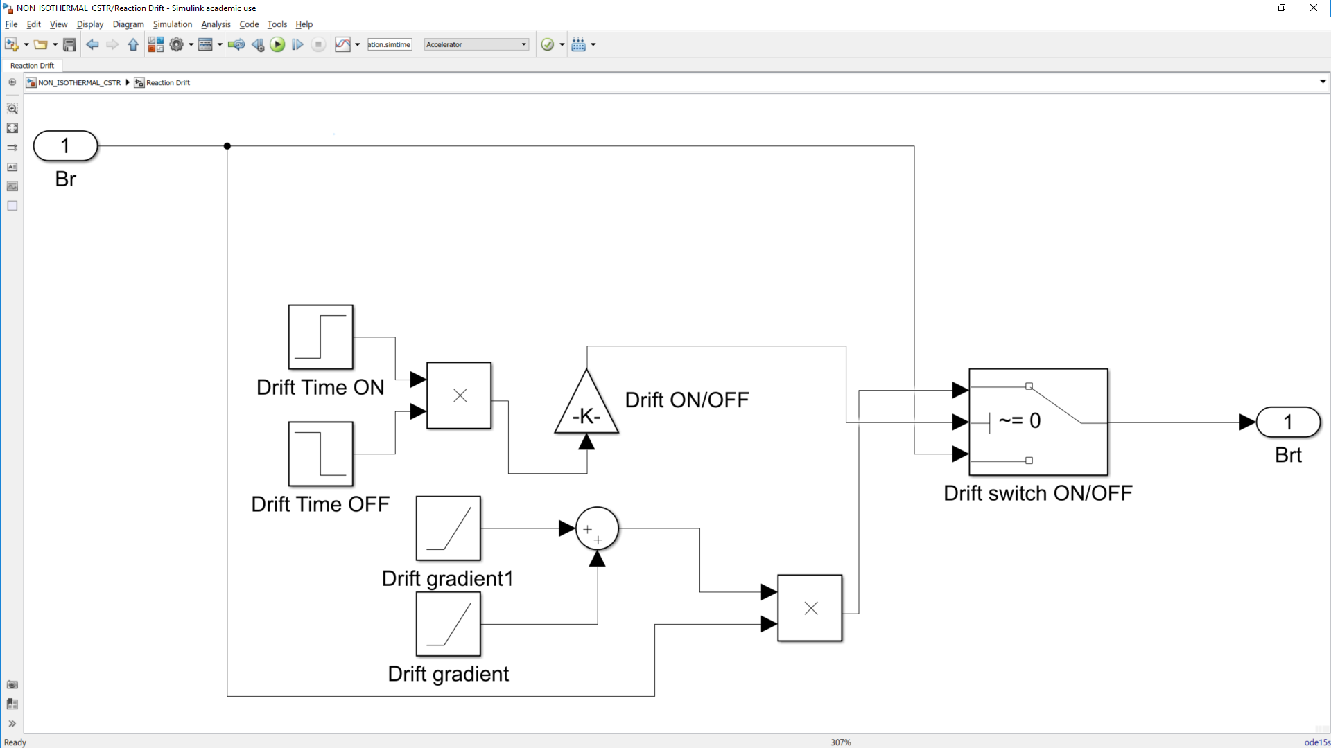
Figure 1.2: Reaction drift model.

Multimodal operation

Multiple mode operations are introduced as a change in product specifications. This is modeled as changes in controller set points of the controlled variables. Mode changes are activated by causing step changes in either the concentration or the temperature set points at specific time intervals. The modeling as shown in Figure 1.3 presents a view of how the set points are passed to the controller. It can be seen as the primary set point (one) is passed unless set point two is activated, then set point two is passed. For each multimodal option, a total of three set point changes can be effected and consequently four operation modes can be achieved.

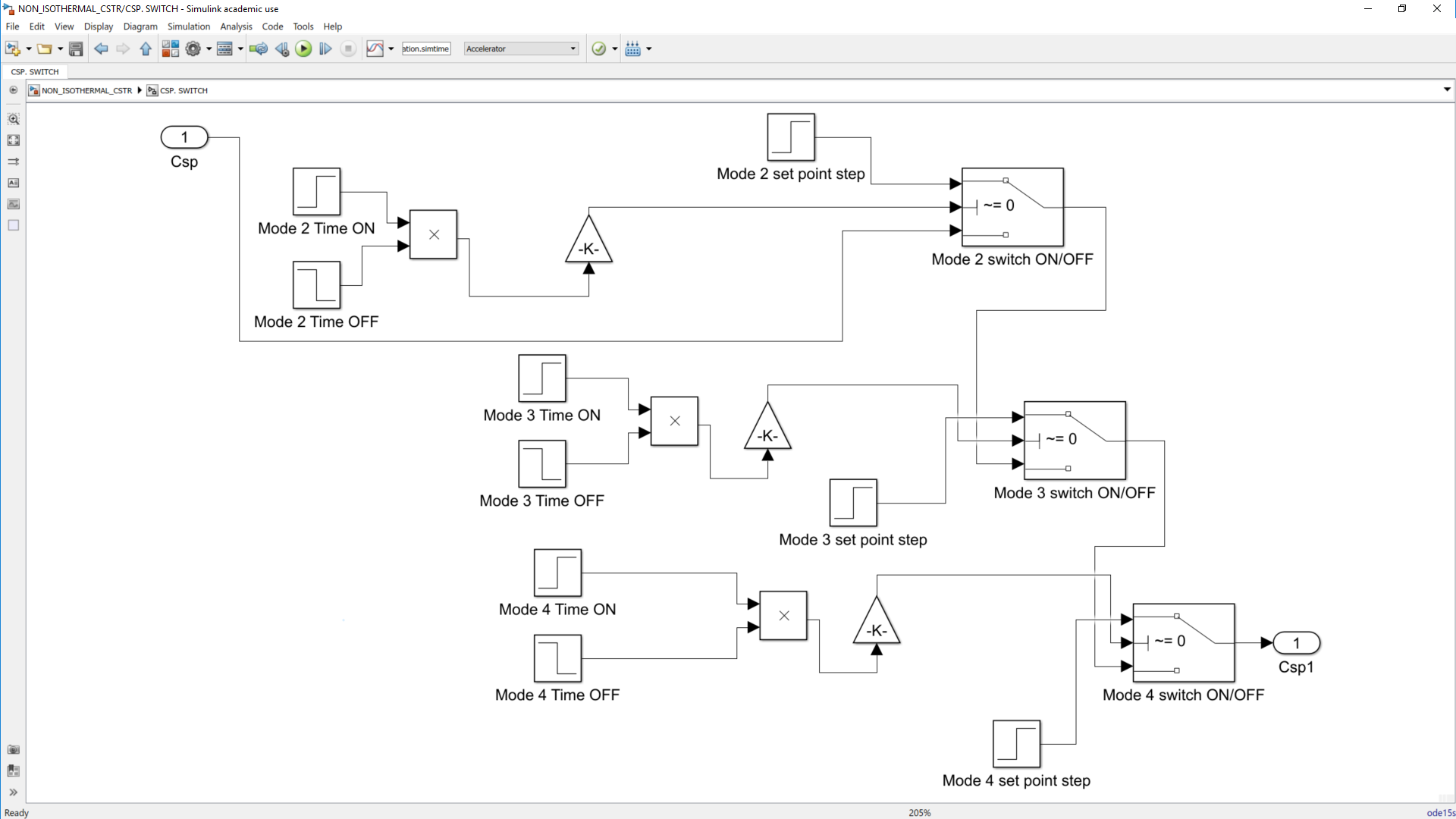
Figure 1.3: Mode changes as a step change in concentration controller set point.

Process inputs

As mentioned earlier, all process inputs are modelled as a first order AR processes as shown in Figure 1.4.

The overall model involves a tapped delay in the variable and the relevant AR coefficient, measurement noise and the constant term that makes sure the input does not have zero mean. The associated switch is an implementation of the step fault in the process input at a specific time. The general process faults are described in the subsequent Section.

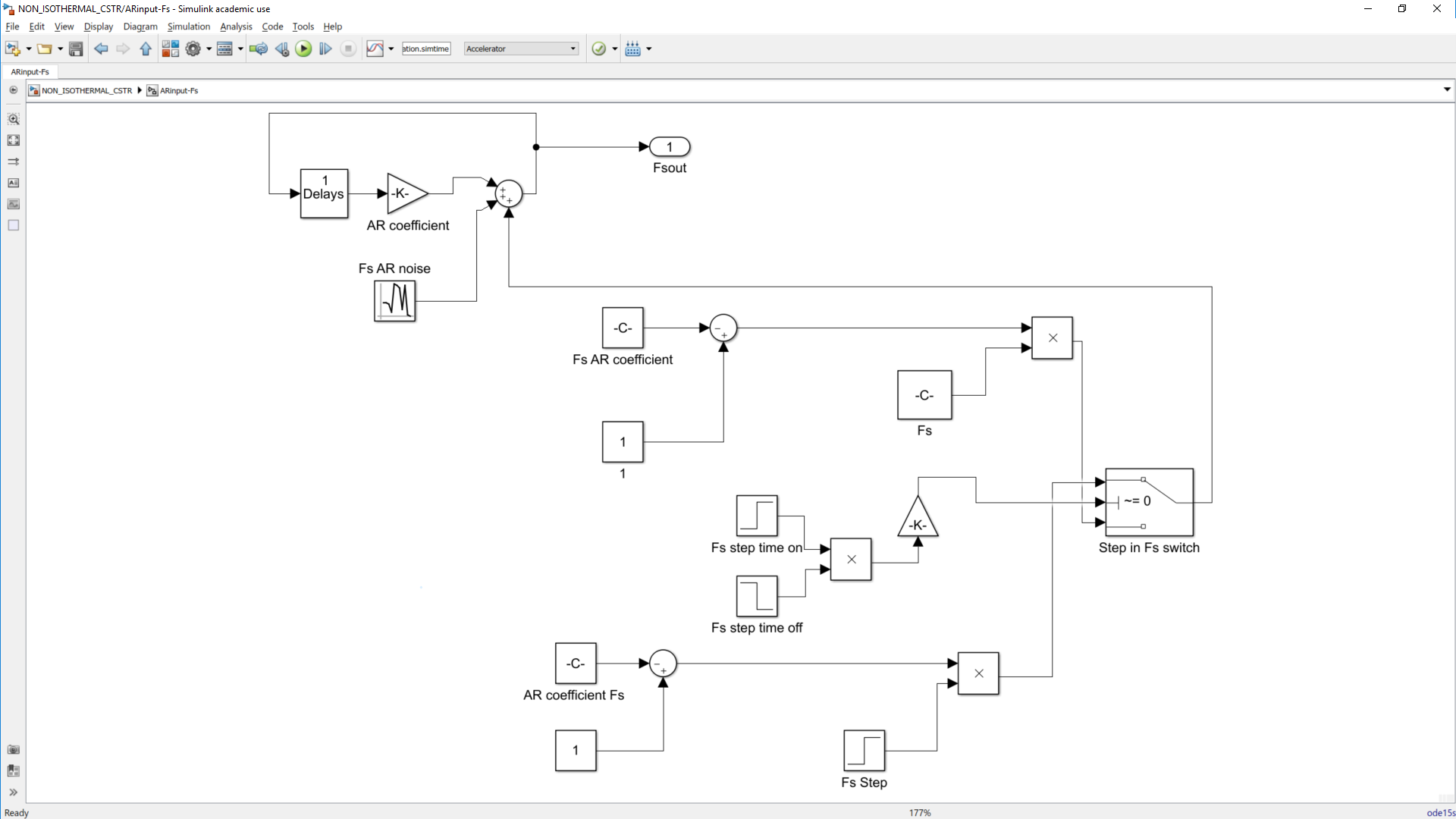
Figure 1.4: An autoregressive process model for Fs input.

Process faults

The model incorporates three distinct faults, namely sensor drift faults, sensor bias faults, and process input step faults. While sensor drift and sensor bias faults are modeled for all the nine measured variables, the input step faults are available for the seven process inputs. Two of the step input faults, the step in F_c and F_a, can only be implemented when the temperature controller and concentration controllers are respectively off.

The sensor drift faults as shown in Figure 1.5, are ramps with specific times to be implemented. Sensor bias fault and sensor drift fault in the same variable can only be implemented one after the other. If both sensor bias and drift fault in the same variable run simultaneously, only the sensor bias fault is implemented.

Classification of the process faults as simple or complex depends on the way the fault propagates in the system. A simple fault is reflected in only one variable, while a complex fault is reflected in an impact on other variables (Yoon and MacGregor, 2001; Mnassri, El Adel and Ouladsine, 2015). An example of a complex process fault is a step input in C_s which impacts the reactor concentration and forces the reaction of F_a in a closed loop process. A sensor bias or drift fault in C_s is classified as a simple fault because it only affects the variable C_s. Table 1.6 provides a summary of all the modeled faults and their respective classifications. The faults registered as complex/simple refer to faults which are complex when the controllers are activated and simple when the controllers are deactivated.

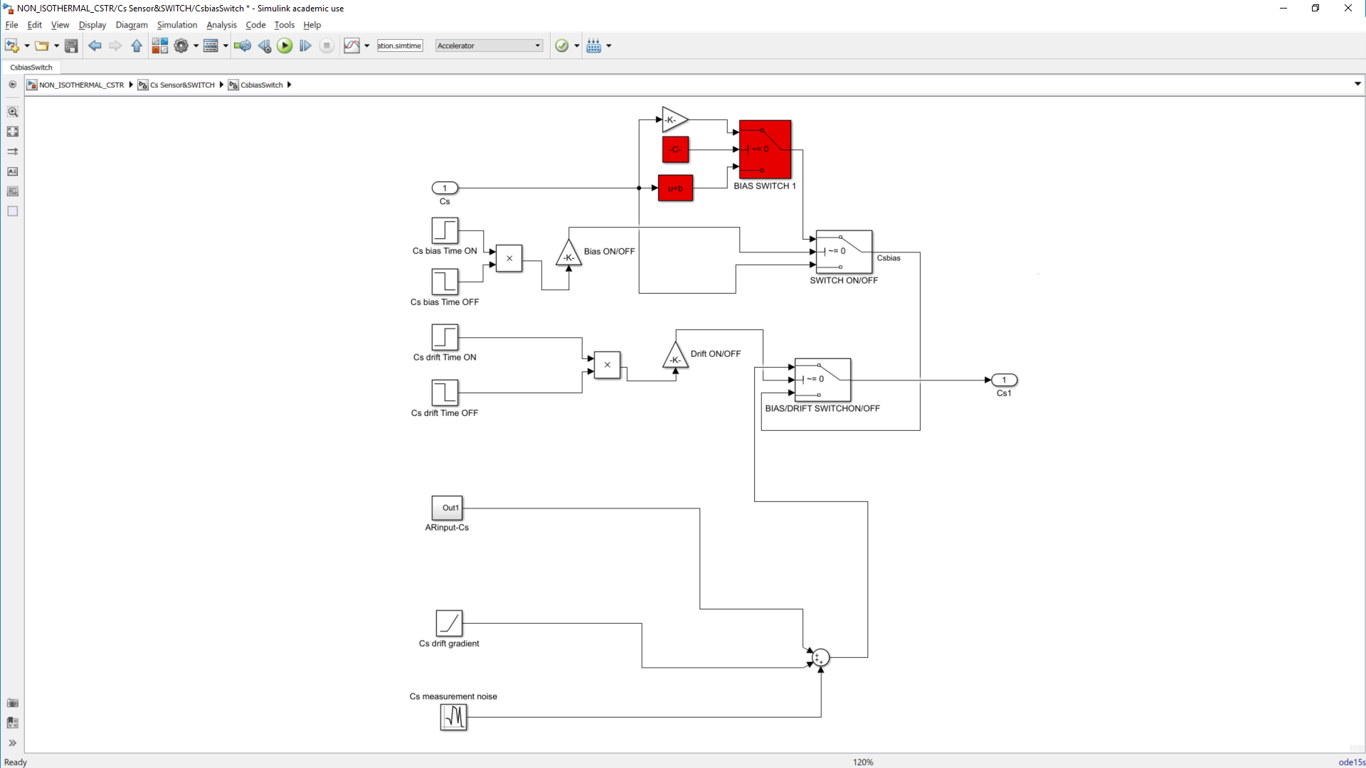
Figure 1.5: Sensor bias/drift fault in Cs model (red highlights addition of bias as a fixed value).

Table 1.6: Summary of fault descriptions as simple or complex faults.

Variable	Input step	Sensor Drift	Sensor Bias
F_s	complex	simple	simple
T_i	complex	simple	simple
T_c	complex	simple	simple
C_s	complex	simple	simple
C_a	complex	simple	simple
F_c	complex	simple	simple
F_a	complex	simple	simple
T		complex/simple	complex/simple
C		complex/simple	complex/simple

The overall process of complex and simple faults modeling for the sensors can be seen as shown in Figure 1.6 where the sensor measurements are passed into the process for variables highlighted green and red for not passed. The difference is treating sensor faults as measurement faults that do not affect the actual process, unless in the case whereby the variable is controlled which involves reaction from the controller involved then it becomes complex.

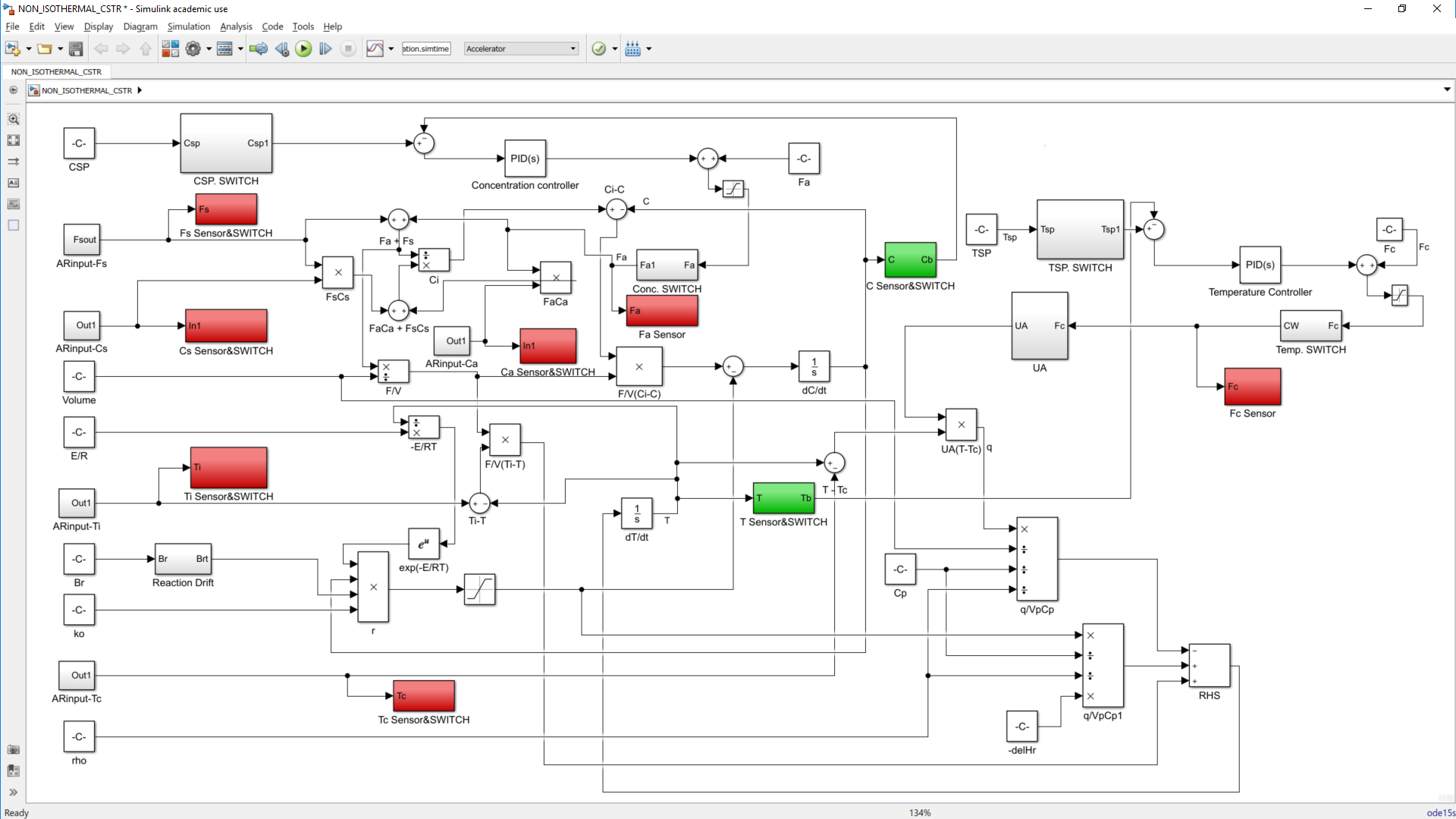
Figure 1.6: Complex/simple sensor drift/bias faults. (Red color refers to simple faults while green highlights complex faults).

Controllers

The model provides concentration and temperature controllers which are PI controllers that can be implemented in a closed loop simulation. The controller implementations are such that the allowable maximum number of inactive controllers is two for unimodal, and one for multimodal. This is a result of the need for a controller to cause the mode changes as described by the change in controller set points.

Seeds

All process and measurement noises make use of a random number generator, with the seeds of the random number generators being unique for the individual noises as well as each simulation.

The MATLAB program consists of the ‘CSTR_simulator’ script that opens up the ‘NON_ISOTHERMAL_CSTR’ Simulink file and provides the user with a number of Graphical user interfaces that takes required information for the simulation and saving of the simulated data. The relevant simulation details required are the simulation parameters, simulation and sampling time and controller details for closed loop simulation. Another required information is for faults and their respective times in test data generation.

The various information required are captured in each user interface are presented in the subsequent sections.

Generally, all interactive fields at each point have green backgrounds and can either be a button, drop-down menu, a text field (for entering a value) and table (with editable fields). Anything with a grey background is just a placeholder and perform no action.

Please make use of the ‘close’ options provided in the program to exit figures, only close the MATLAB figures using the MATLAB in-built button when it is the only option.

Home Parameters Simulation types Data Simulation specifications PI controllers Reaction drift Fault specifications Summary Results Saved data

The ‘Home’ page (shown in Figure 1.7) is the first page after running the ‘Reactor_simulator’ script. It provides two buttons with options to specify reactor parameters from scratch or load the default parameters and edit the required fields.

Clicking on either button opens the respective pages for load default parameters and the new reactor parameters. To exit the home page, the figure must be closed.

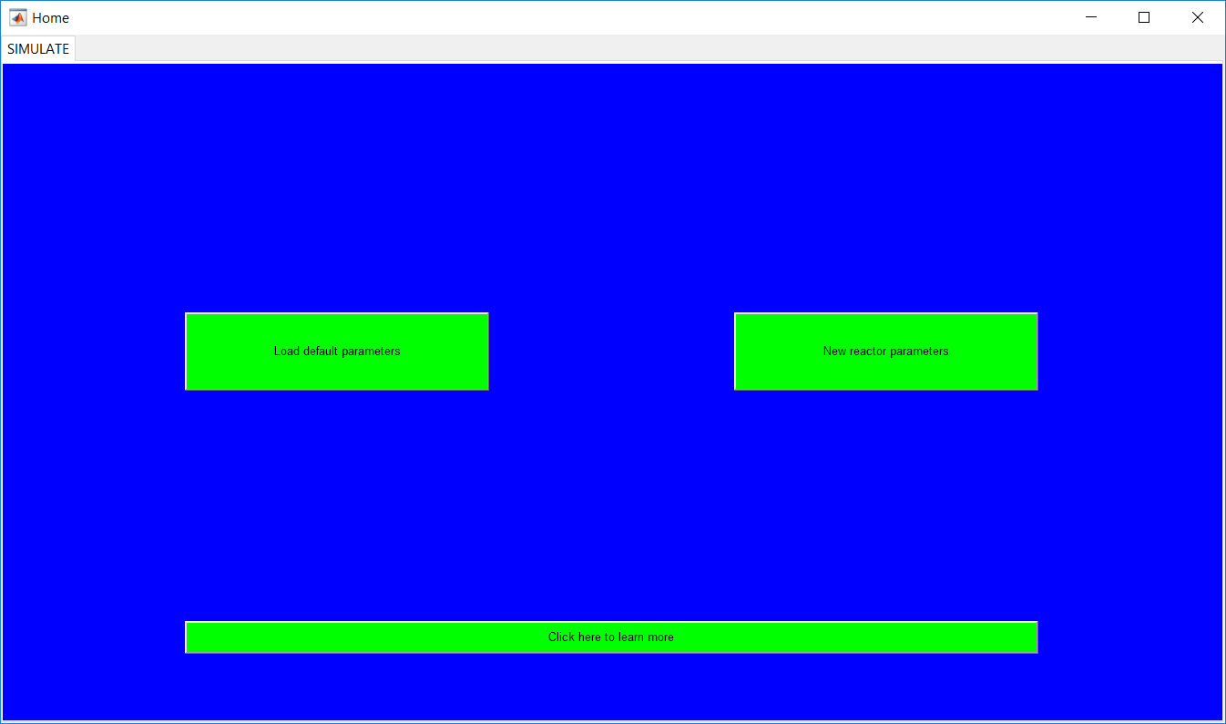
Figure 1.7: Home page.

Load default parameters

Selecting the option to load default parameters opens up the ‘Reactor Parameters’ page shown in Figure 1.8 which contains a table preloaded with parameters values described in the previous sections and an editable ‘value’ Section column. The only form of data validation for the values are checks for numeric inputs in the fields. This involves resetting the changed value to pre-existing value if conditions are not met and a warning sign that pops up to alert the user.

Inputs are saved by clicking elsewhere in the page after keying in a value or alternatively hitting the return/enter key.

The ‘Reload’ button restores the table to its initial state and discards any user input.
The ‘Confirm’ button saves the reactor parameters and continues to the ‘Simulate types’ page.

Although values for the parameters of the PI controllers are required to be provided, the values keyed are not critical if an open loop simulation is needed since options to disable the respective controllers are presented in the ‘Simulation specifications’ page.

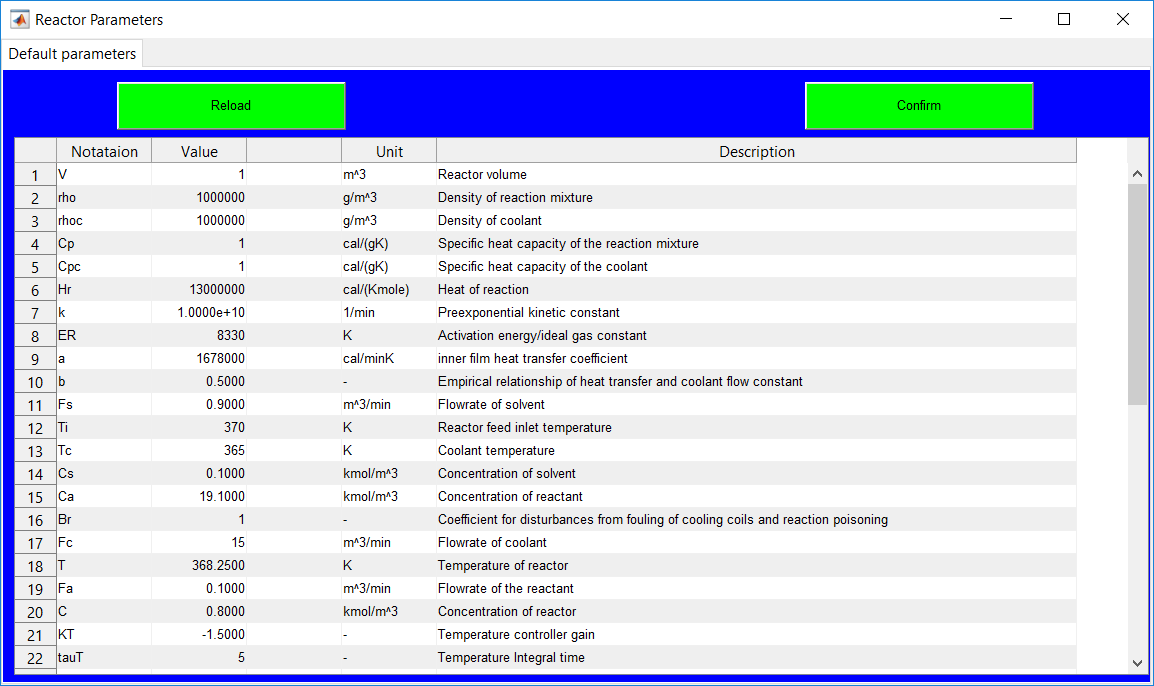
Figure 1.8: Reactor parameters page for selecting the option to load default parameters.

New reactor parameters

Selecting the option to provide new parameters opens up the ‘Reactor Parameters’ page with the same description like that for the default parameters but with no preloaded reactor data as shown in Figure 1.9. The ‘value’ column Section rather contains ‘click to input’ texts that need to be cleared for specific inputs to be made.

The ‘Go back’ button closes the existing page and returns the user to the ‘Home’ page.
The ‘Refresh’ button, discards all changes made and presents the initialized table data.
Until all the fields are appropriately completed, the ‘confirm’ button remains pops up a warning requesting that all fields must be completed. It, however, continues to the ‘Simulate types’ page if all inputs are validated as correct.

As with the ‘load default parameters’ page, a ‘Specify parameters’ message box is associated with the page provides information about the buttons.

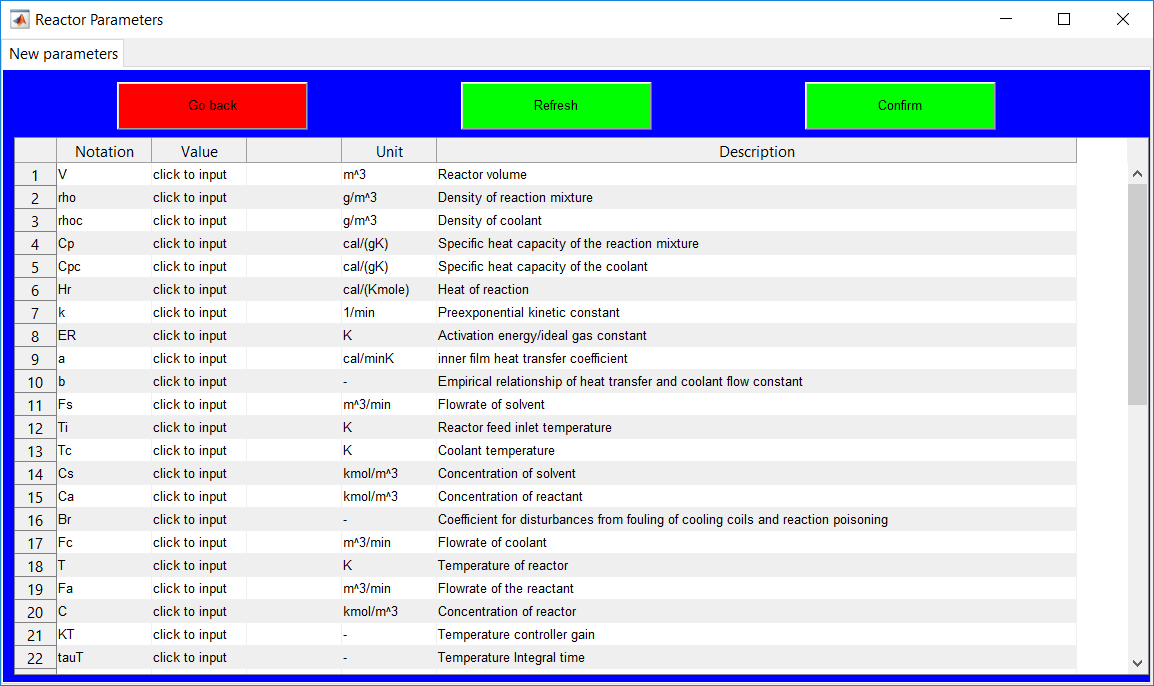
Figure 1.9: Reactor parameters page for selecting the option to load specific parameters.

The ‘Simulation types’ page shown in Figure 1.10 provides options to select the data type to generate.

The ‘Training data’ button provides options to simulate data free of faults.
The ‘Validation data’ button provides the same options as the ‘Training data’ button in generating fault-free data.
The ‘Test data’ button provides the same options as the two other buttons but with an extra information about faults to generate in subsequent pages.
The ‘Go back’ button returns the user to the ‘Reactor Parameters’ page which is the previous page.

Selecting any of the three data generation buttons on the page opens a pop-up menu that requires the user to specify whether unimodal or multimodal data is to be generated.

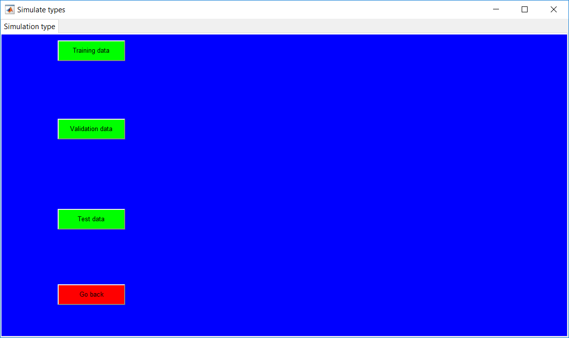
Figure 1.10: Simulation type page.

Unimodal/multimodal

The options to simulate a multimodal or unimodal process is provided in the drop-down list as shown in Figure 1.11. Information about the mode types is passed by clicking on the appropriate mode selection from the list.

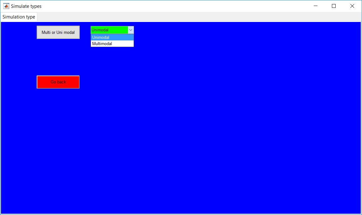
Figure 1.11: Unimodal/multimodal pop-up menu.

The unimodal option opens the unimodal section.
The multimodal option also opens up the multimodal section.
The ‘Go back’ button returns the user to ‘Simulate types’ page.

Unimodal

Selecting the unimodal option from the drop-down list opens the green button as shown in Figure 1.12 which provides an option to continue.

The green button proceeds to ‘Simulation specifications’ page for validation and training data (presented in Section 4.10).
The green button proceeds to the ‘Fault specifications’ page for test data.
The ‘Go back’ button returns the user to ‘Simulate types’ page.

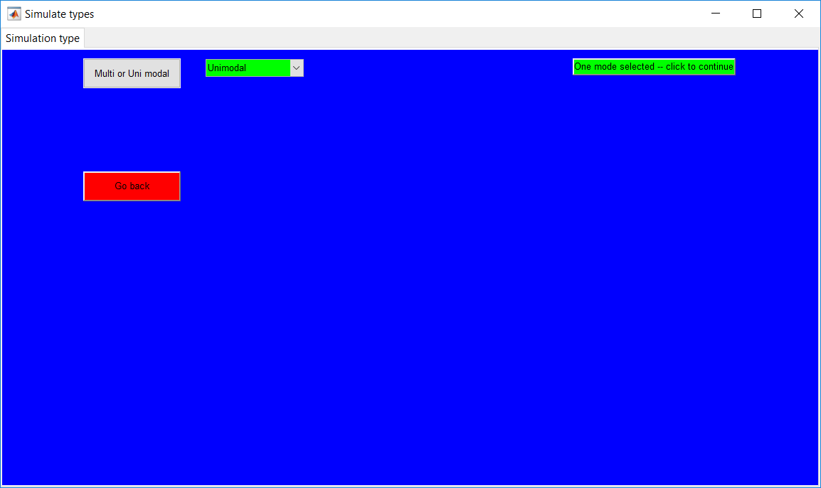
Figure 1.12: Unimodal simulation selected page.

Multimodal

Selecting the multimodal option opens a pop-up menu that provides an option to select change in modes as concentration (C) controller or Temperature (C) controller set point change as shown in Figure 1.13. The ‘variable to change’ message box also provides information about the options in the drop-down list of the pop-up menu.

Selecting either option opens another pop-up menu that requires the number of modes to simulate.
As with the unimodal simulation, the ‘Go back’ button returns to the ‘Simulation types’ page.

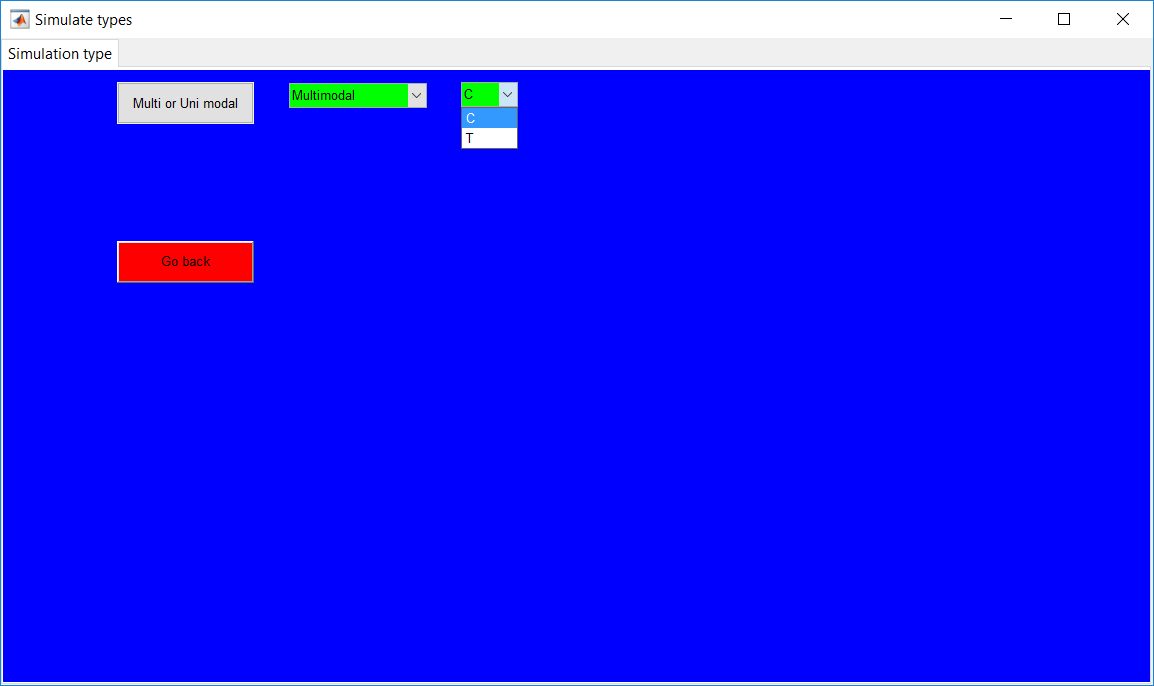
Figure 1.13: Multimodal simulation selected page.

Number of modes

A maximum of four modes can be simulated as shown in Figure 1.14. Selecting any number of operating modes opens up the option to specify the set points of the modes.

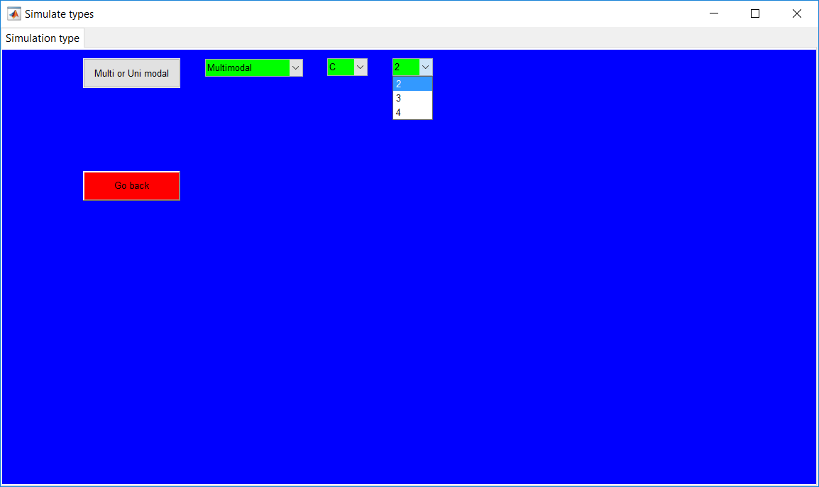
Figure 1.14: Selection of number of modes to simulate.

Set points

The new set points of the controllers are required to be specified in percentages of the first set point value as shown in Figure 1.15. To provide an idea of the current set point, an information box displays the current set point which is the steady-state value of the variable. The other options with ‘Enter mode set point’ are to be cleared and a set point value to be entered. For example, to change the set point of the concentration controller from 0.8 to 1.2, the value of 150 is entered into the designated field.

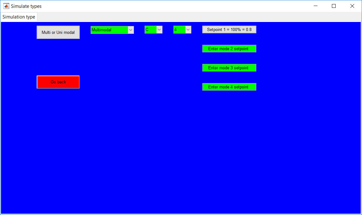
Figure 1.15: Option to enter new set point values.

An option to continue to the ‘Simulation specifications’ page for the multimode process is provided for training and validation data simulations once all fields are validated for numeric inputs as shown in Figure 1.16.

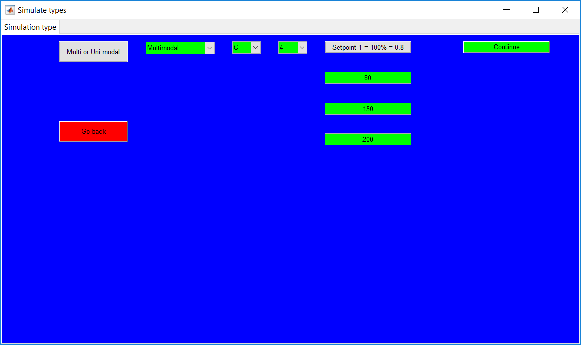
Figure 1.16: Option to continue to after entering new set points.

In contrast to the training and validation data, comp leting the required fields for the test data opens up the ‘Fault specifications’ page.

Unimodal training/validation data

The ‘Simulation specifications’ page (in Figure 1.17) for unimodal training and validation data provides options to specify the details of the simulation duration and the sampling time. The total number of data points generated is evaluated as the simulation duration/sampling time.

Completing the required fields for the simulation and sampling times opens a button that provides a user with a ‘Summary’ page.

The times are specified by clearing the ‘Enter value’ Section and inputting the appropriate
‘Reaction upgrade/degrade’ button provides options to activate/deactivate the reaction drift.
Buttons with ‘Click here to turn on/off’ provide options to activate/deactivate the PI controllers.
The ‘Go back’ button returns to the ‘Simulation types’ page.

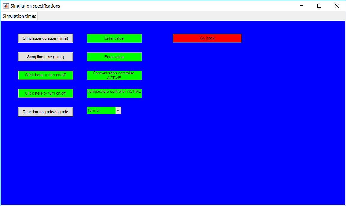
Figure 1.17: Simulation specifications for time specifications – Unimodal.

Multimodal training/validation data

The ‘Simulation specifications’ page for multimodal training and validation data as shown in Figure 1.18 provides the same requirements as the unimodal section with extra specifications for times to switch from one mode to another.

All mode change times and the required fields for the simulation and sampling times need to be completed before an option to the ‘Summary’ page is provided.

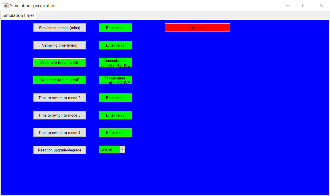
Figure 1.18: Multimodal simulation specifications page for training/validation data.

Multimodal/Unimodal test data

The ‘Simulation specifications’ page (shown in Figure 1.24) for test data has the same features as that for the training/validation data with extra options to specify the time details for the selected faults.

All controllers can be activated/deactivated for all unimodal data simulation types as shown in Figure 1.19. This is achieved by clicking on the buttons beside the respective controllers to change the current state. For multimodal simulation, on the other hand, a maximum of one controller can be deactivated as shown in Figure 1.20. The controller fixed to achieve multimodal simulation cannot be deactivated. The ‘Warning’ message pops up when the fixed controller is clicked and remains unaffected.

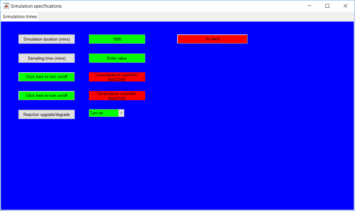
Figure 1.19: Unimodal simulation controller options.

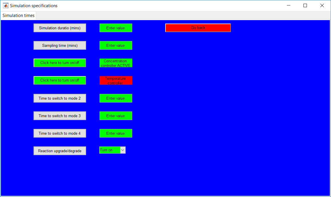
Figure 1.20:Multimodal controller activation/deactivation options.

The reaction drift option, as described earlier, provides options to degrade/upgrade reaction performance. Options to turn on/off the drift is provided by selecting from the drop-down menu right to the ‘Reaction upgrade/degrade’ button as shown in Figure 1.21.

A positive drift is implemented by moving the slider originally at zero position to the right and the reverse for negative drift.
The ‘drift start time’ and ‘drift end time’ provides options for times for implementation of the drift.

Figure 1.21: Reaction drift selection and specification option.

Upon completion of the required fields for the drift, the current drift rate is provided in the text field below the slider as shown in Figure 1.22. The drift rate is computed as magnitude/(start time- end time).

The magnitude is attained by moving the slider with the maximum positive and negative drifts as one.
The ‘Continue’ button provides a link to the summary page.

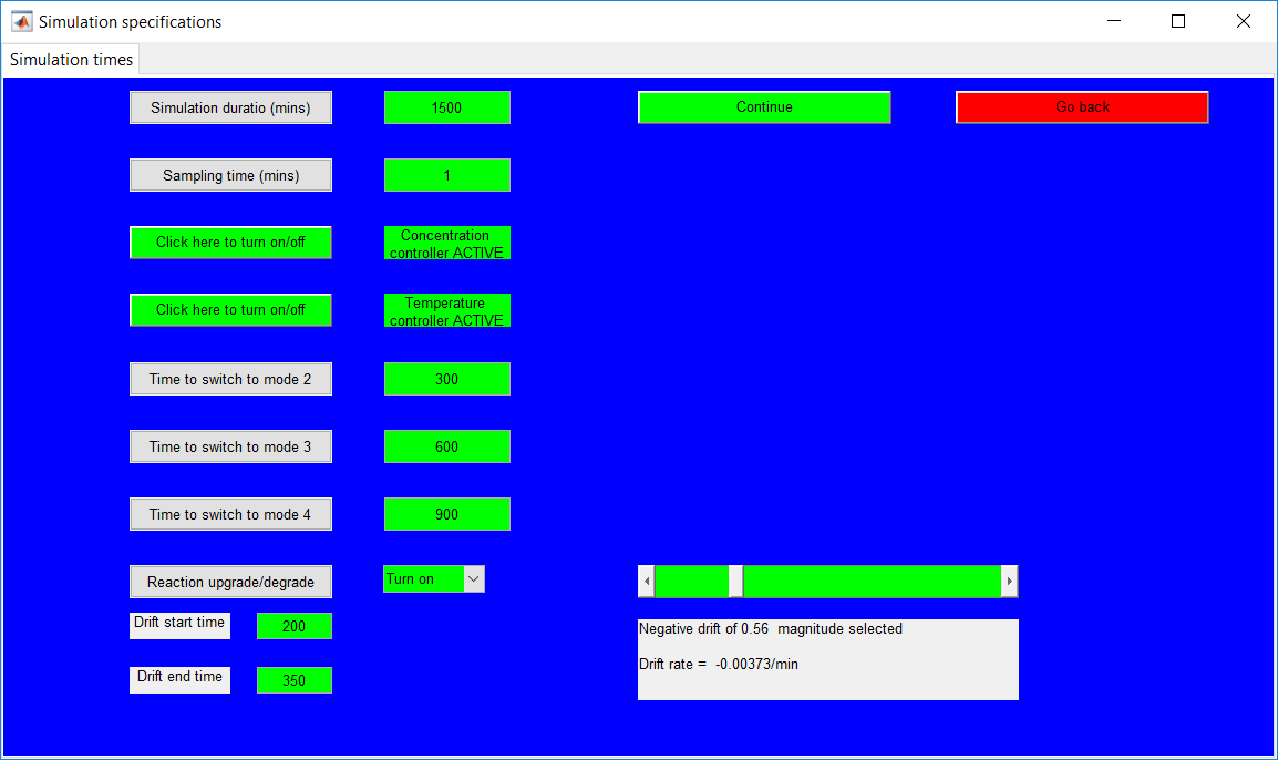
Figure 1.22: Selected reaction drift rate at specified times.

The ‘Fault specifications’ page collects information about the respective faults to be simulated for test data as shown in Figure 1.23. The faults are activated/deactivated by clicking the respective on/off buttons.

The sensor bias faults are to be specifed as percentages of the original sensor readings.
As with the sensor bias faults, step input requires step values to be specified as a percentage of the initial value. The ‘faults’ message box also provides information about how to input respective faults.

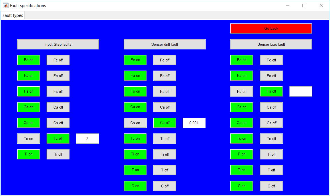
Figure 1.23: Fault specifications page for test data.

Simulation specifications

The final step value/sensor bias values are computed as (1 + input value/100) × initial values/sensor readings.

While sensor drift and bias faults can be implemented in all variables, activating the input step in the manipulated variables pops up ‘Fc warning’ and ‘Fa warning’ message boxes respectively for the Fc and Fa step faults. This is as a result of the two controllers being active by default, and if not deactivated the respective step input faults would be overridden.

The selected ‘fault on’ and ‘fault off’ which require the times to activate and deactivate the faults. Completing all specified fields opens up the ‘Summary’ page.

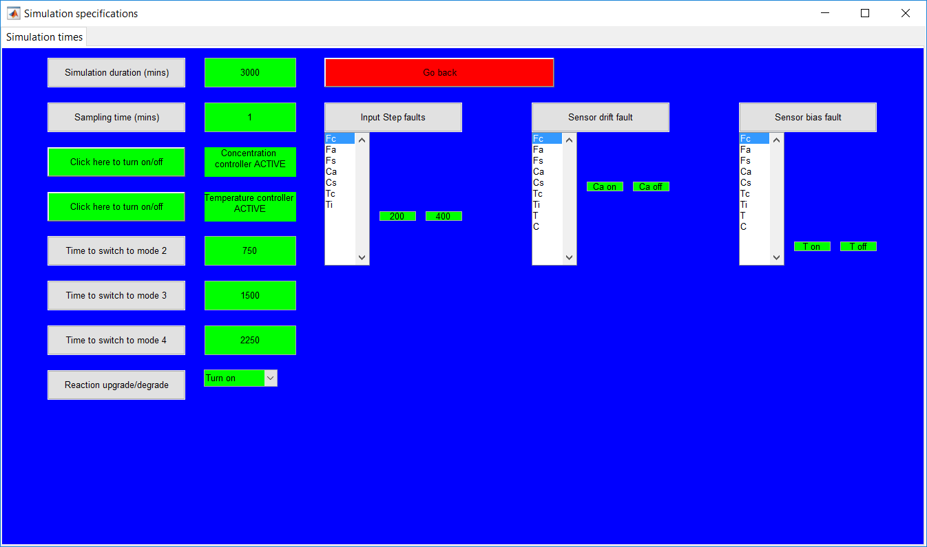
Figure 1.24: Simulation specifications for test data.

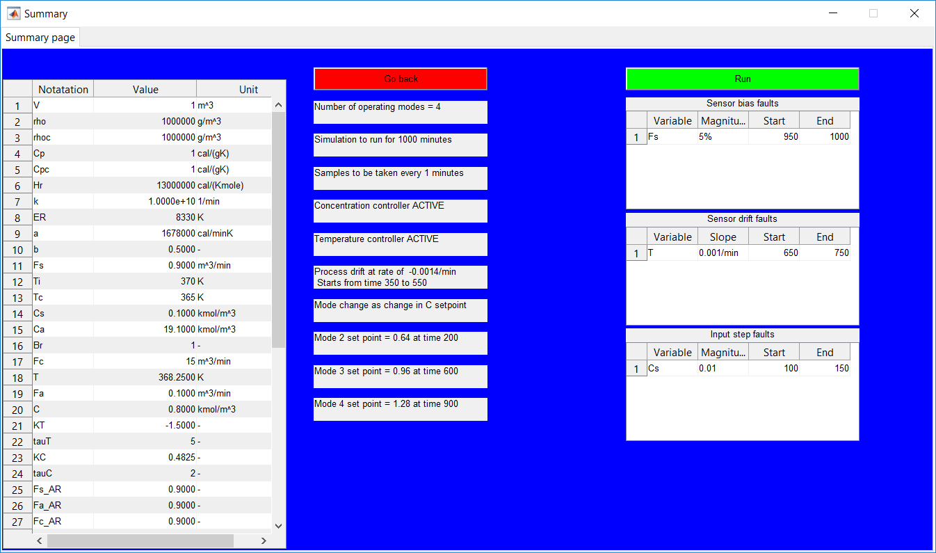
The ‘Summary’ page provides a summary of all the information given by the user as shown in Figure 1.25. Test data simulation provides additional information about the selected faults to be implemented at specific times and magnitudes.

The ‘Run’ button simulates the non-isothermal CSTR model using the information displayed on the page and pops-up the ‘Results’ page.
The ‘Simulating’ message box that displays information about the current run is associated with it.

Figure 1.25: Summary page for specified data.

The ‘Results’ page as shown in Figure 1.26 provides a preview of the generated simulation results for all nine process variables.

The ‘Save and exit’ button pops up the ‘Simulation complete’ message box that displays information about the directory to which the data was saved and returns the user to the ‘Home’ page.
The ‘Go back’ button returns the user to the ‘Summary page’ without saving the simulated data.

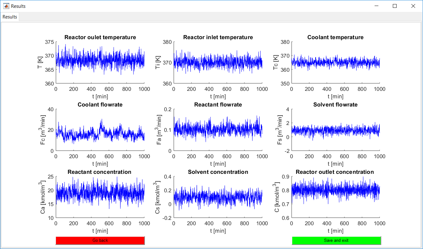
Figure 1.26: Results preview of simulated data.

The ‘Results’ page as shown in Figure 1.27 provides a preview of the generated simulation results for all nine process variables.

The ‘Save and exit’ button pops up the ‘Simulation complete’ message box that displays information about the directory to which the data was saved and returns the user to the ‘Home’ page.
The ‘Go back’ button returns the user to the ‘Summary page’ without saving the simulated data.

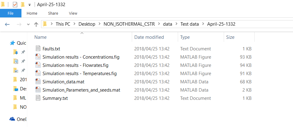
Figure 1.27: Information about the saved simulation data.

Process Monitoring Toolbox

This work builds a toolbox that employs principal component analysis (PCA), adaptive PCA (APCA) as well as Gaussian mixture models (GMM) and adaptive GMM techniques. Moving window PCA (MWPCA) and recursive PCA (RePCA) are the APCA techniques available. The toolbox supports model training, validation, and testing for various data types and faults. The unique approaches available are PCA, MWPCA, RePCA, GMM, and adaptive GMM. Dynamic PCA can also be achieved by lagging the data when performing PCA. For the GMM methods, the decision on the data type (whether scores, normalized or raw) is only available after selecting either approach.

The information presented in the subsequent pages assume that you have a fair knowledge of PCA and GMM and their respective terminologies. If not, click here for an excerpt from Prince Addo’s (my) thesis. Please note that some wordings may be out of place.

The general pages are the pages common to all methods and it is advisable to look at the PCA method before the other techniques as all other methods build on it. Also, some general information which might be needed elsewhere is contained in the PCA pages only.

Please make use of the ‘close’ options provided in the program to exit figures, only close the MATLAB figures using the MATLAB in-built button when it is the only option.

If in need of some data, you can visit the UCI Machine Learning Repository. Also, the MATLAB version of the Tennessee Eastman process data can be downloaded here.

Software requirements

Users with MATLAB app version R2014b and above can install the ‘Process Monitoring Toolbox.mlappinstall’ which is a MATLAB app. All other users must install the ‘MyAppInstaller_web.exe’ which is a windows app.

Irrespective of the method selected, some information need to be provided which is generic. Some of these include the data, trained model (if a model is saved and needed to be loaded at a different time for validation/testing), and faults (for test data).

Generally, all interactive fields at each point have green backgrounds and can either be a button, drop-down menu, a text field (for entering a value) and table (with editable fields). Anything with a grey background is just a placeholder and perform no action.

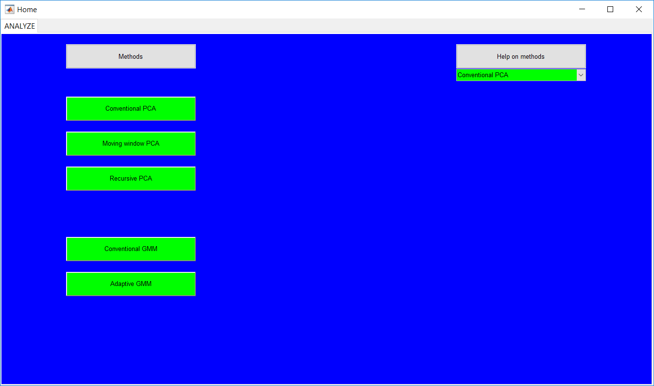
Home Method Data edit Save/Load trained model Fault specifications

The home page displays information about all available methods. The PCA methods are thoroughly listed while the GMM methods are grouped as GMM and adaptive GMM. Either of the GMM methods can be selected for further specifications to be made afterwards. The ‘Help on methods’ provides information on the required hyperparameters for each technique.

Clicking on any method opens the ‘Method’ page with the specific method as a tab.

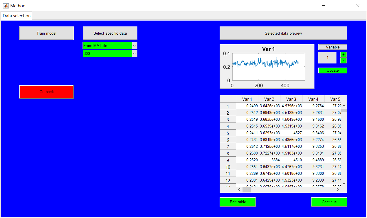
The train model option requests training data to be uploaded by opening the ‘Data selection’ tab on the same page. Specifying to test model or validate model requires a model to be uploaded. Trained/validated models can be saved and later used in the program.

The ‘Data selection’ requires the data to be selected from either the workspace or from a MATLAB file, the uploaded data can be an array or table. The additional drop down to select the specific data is used after the data source (which is either a workspace or MATLAB file) is specified.

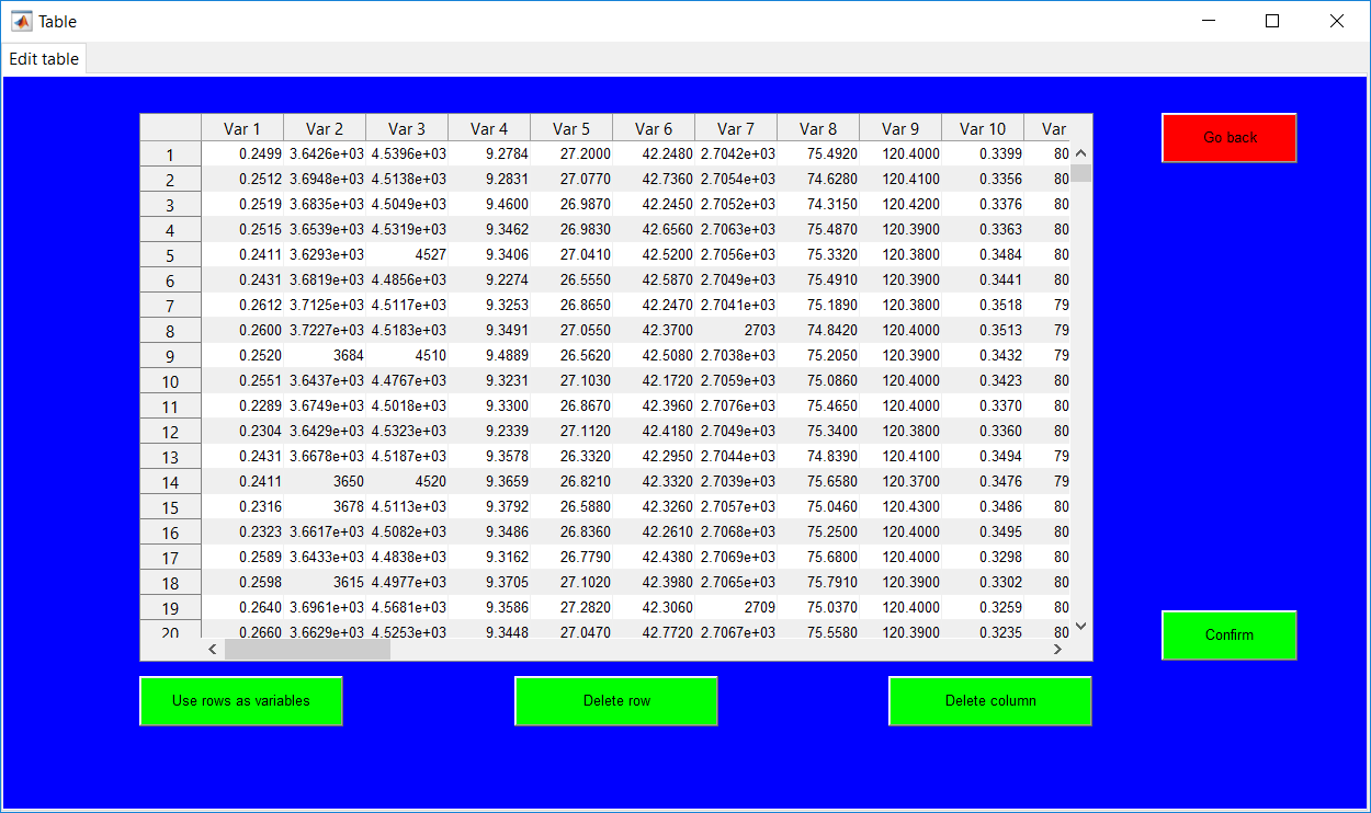
Basic matrix manipulations such as matrix transpose and column/row deletion can be performed using the ‘Use rows as variables’ and ‘Delete row’/‘Delete column’ buttons respectively. Deleting a single row/column requires the number to be specified while deleting a series of rows/columns requires the specification of the first and last values to be removed in the form of a, b with a being the first value. (The operation is guided by the help box).

Going back erases all the changes made to the data and returns to the data preview.

The continue option presents the specific page for the method specified initially, the page is for specifying required hyperparameters.

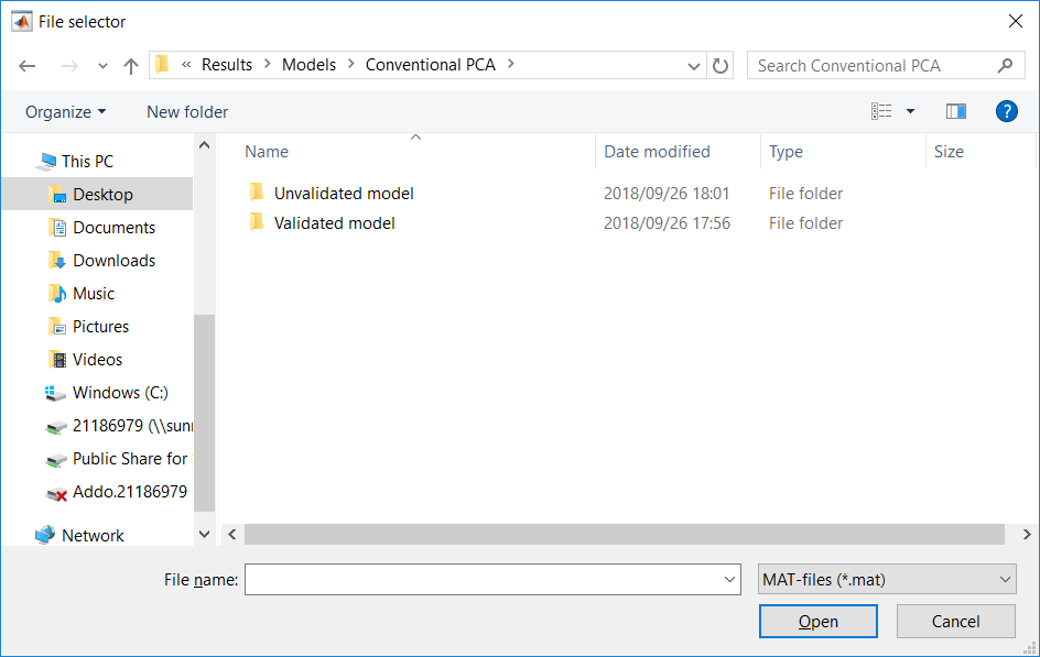
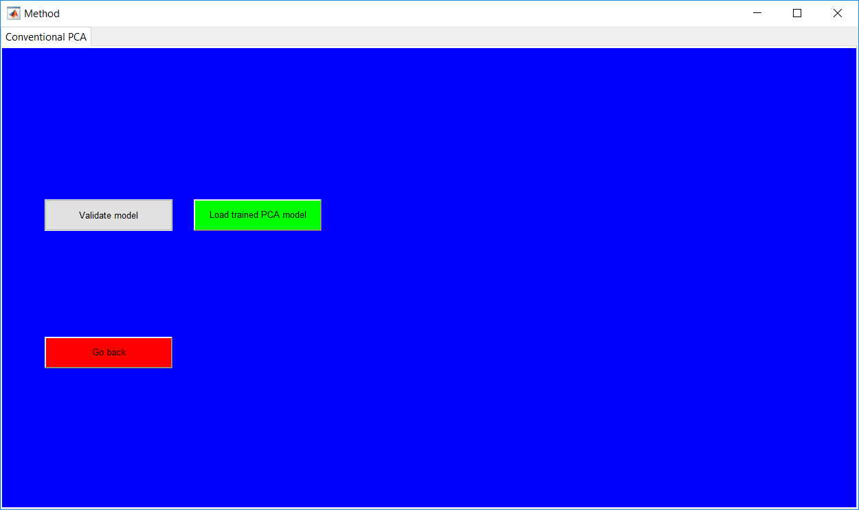
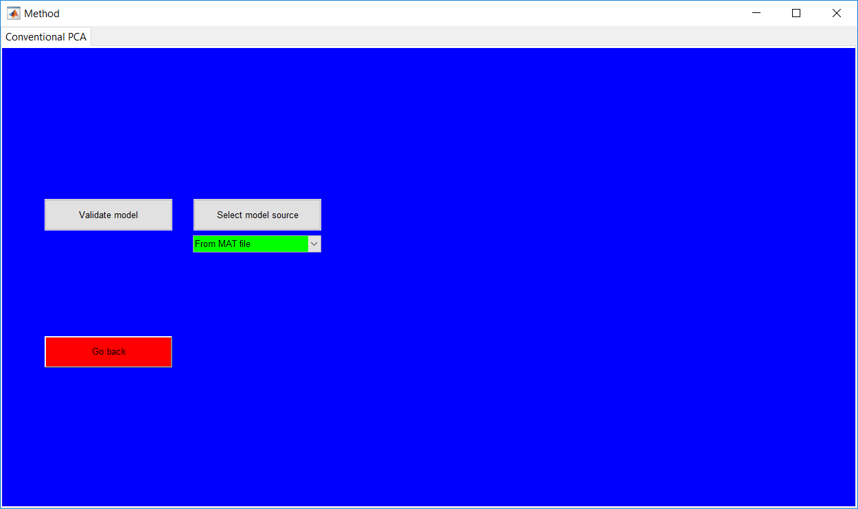
A trained/validated model can be saved and loaded when needed. Un-validated models are saved in an ‘unvalidated’ folder for the respective method. When a trained model is loaded and validated, saving the validated model automatically erases the prior un-validated model from the computer.

Choosing to validate or test trained model on start-up requires the model to be uploaded. Although checks are in place to make sure a model is uploaded instead of a data, the selected model and the desired method to be implemented should be same, i.e. selecting a saved GMM model if GMM is the method to be investigated.

The ‘Data selection’ for the test/validation option is then presented after the model upload.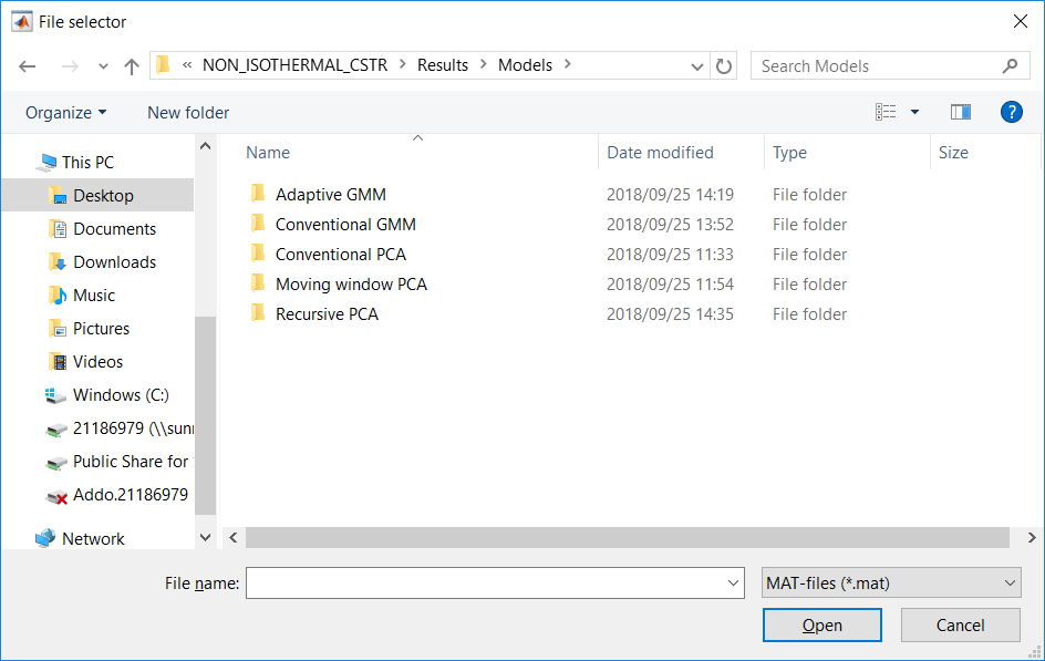

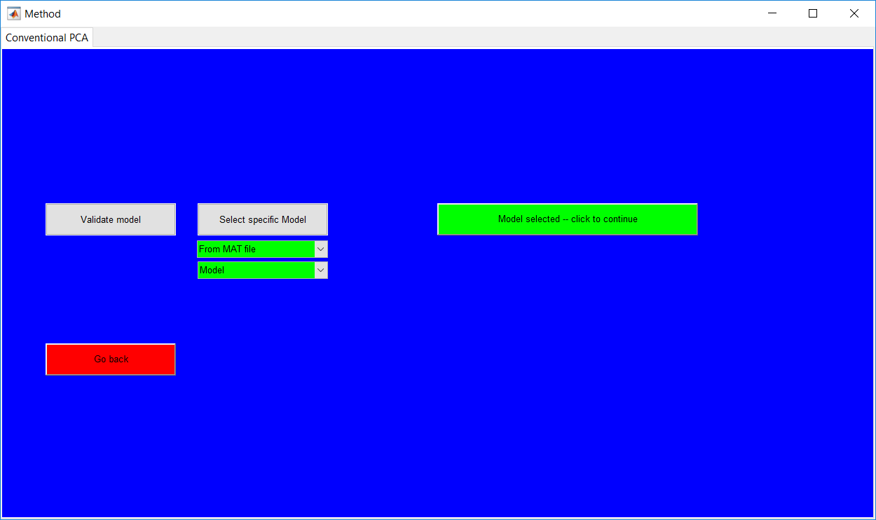
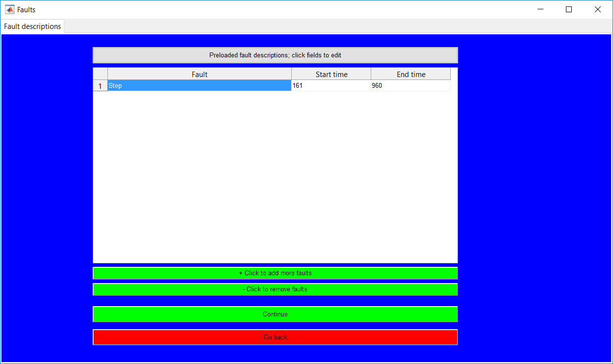
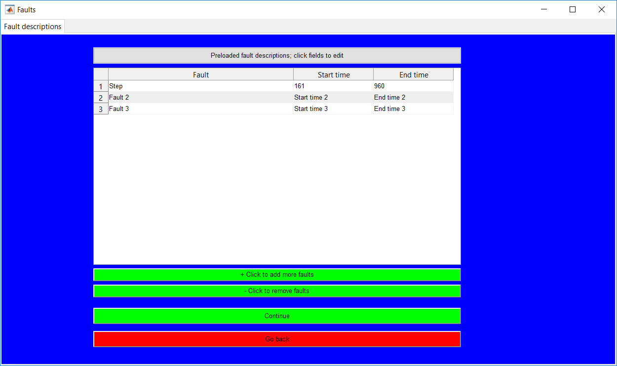
The fault specifications page require information about the known faults, a minimum of one fault needs to be specified (there is no bound on the maximum). If no information of the faults is known, any values in ordered fashion could be entered and the performance metrics consequently ignored or better still make a use of the validation stage instead of the testing.

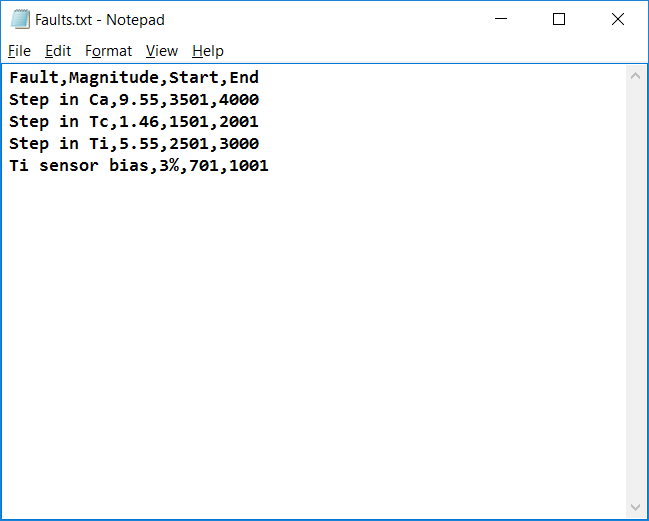
Loading test data from the CSTR model automatically comes with saved fault descriptions which could still be edited. To have the faults to be automatically loaded, a ‘Faults.txt’ file needs to be created with a comma delimiter and specific fields as shown below, the fault and magnitude aspects could be filled with any placeholder as they are not paramount.

Additional faults could be added/removed by using the appropriate buttons provided. In general, the start time for a second fault should not be less than the end time for the previous fault. Also, the end time of a specific fault cannot be less than its start time.

Although there is basic error checking systems in place, the general order should be followed. Continuation of the hyperparameter specifications stage for the test data is only realized if the required fields are duly provided.

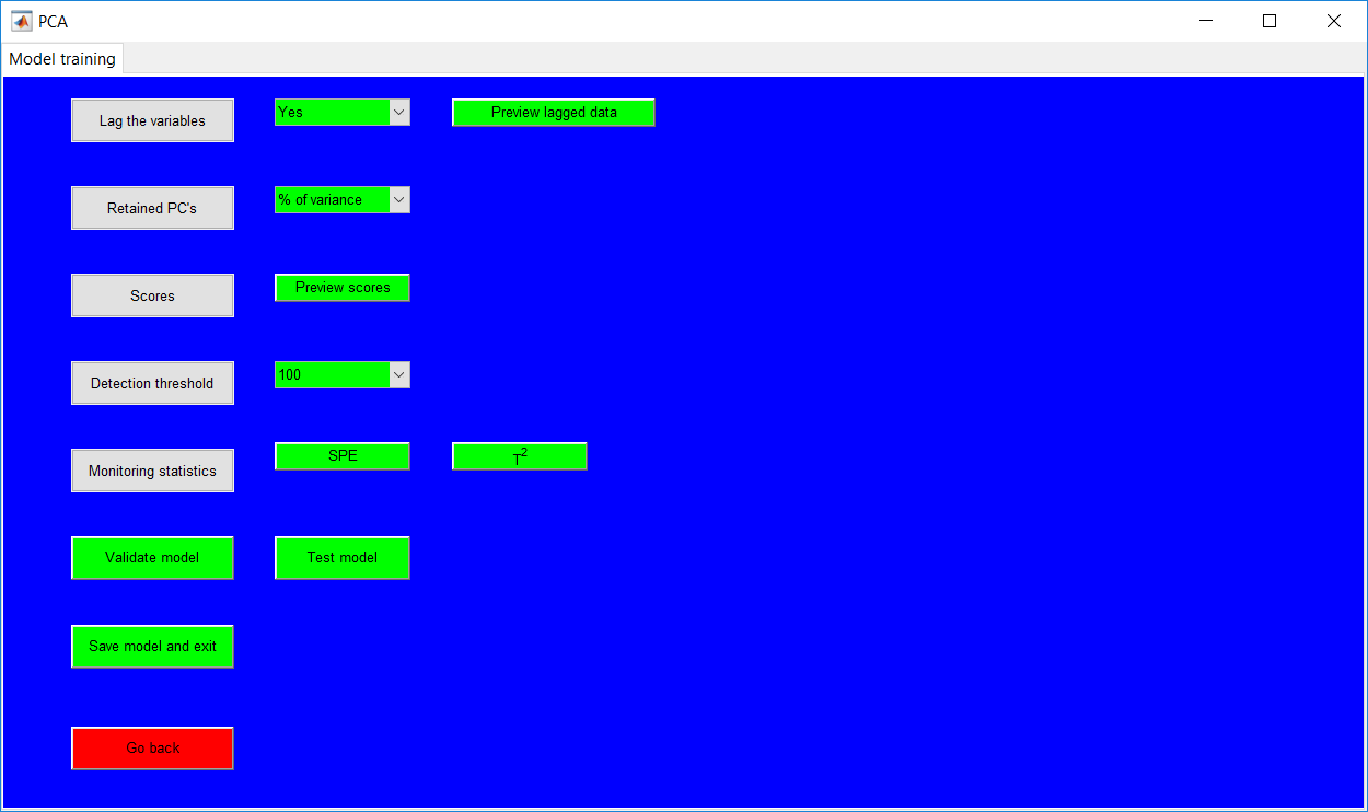
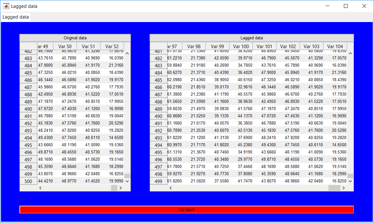
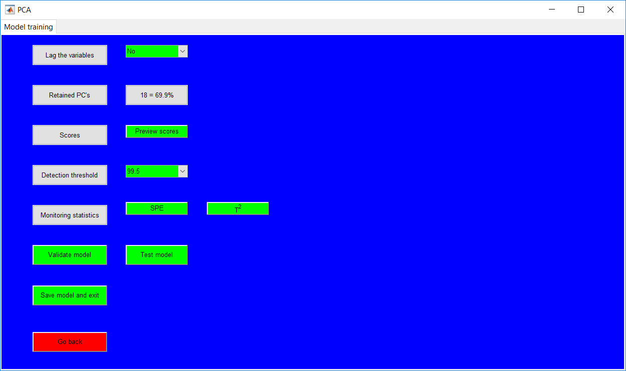
Training page Validation page Test page

The PCA page requires the hyperparameter specifications. A common option for all methods is the option to lag the variables (this is important for implementing dynamic PCA). The default option is ‘No’, and should remain unchanged unless otherwise. If changed, the order of lag is specified as a number (this can be a single negative or positive value). The positive value (lags) correspond to delays and shift a series back in time. Negative lags correspond to leads and shift a series forward in time. If the lag value is appropriately selected, a button for the lagged data preview is provided as ‘Preview lagged data’. This is to provide a display to see if the desired effect is obtained. Generally, the number of observations decrease by the specified order or lag while the number of variables increases by a factor of the lag specified.

Retained principal components

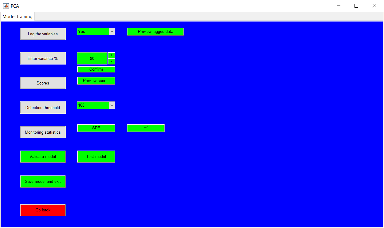
The retained PCs can be specified by selecting a minimum amount of explained variance to retain or a specific number of principal components. The first approach is provided by ‘% of variance’ option which requires the percentage to be specified either by keying in the value or using the provided ‘+’ and ‘-’ buttons. The default value provided after a selection is 50 (%) and using the buttons provide a difference of 5 in either way (i.e. increase or decrease).

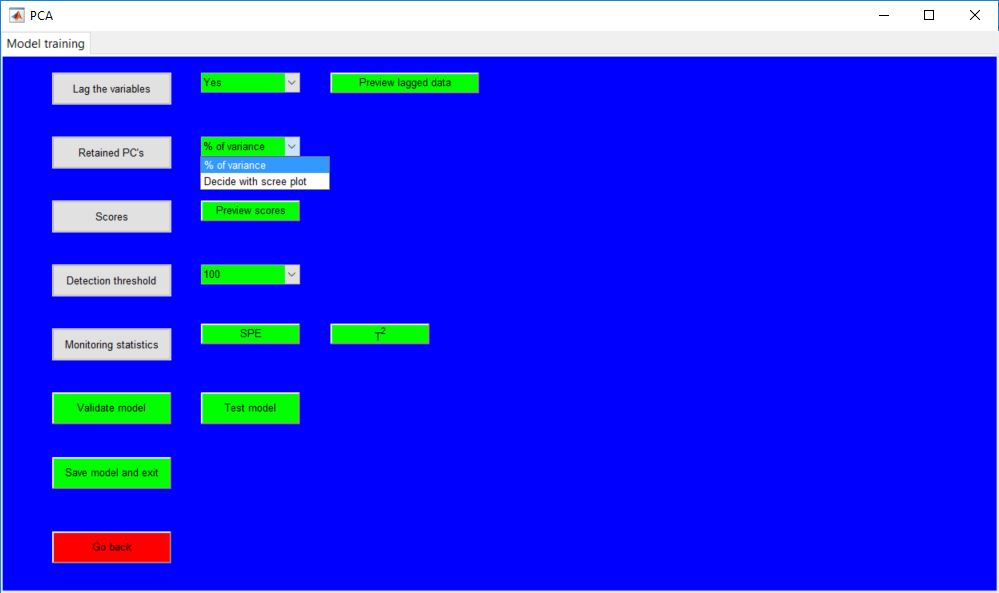
The second option is provided by the ‘Decide with scree plot’. It basically provides a scree plot and a Pareto chart for the principal components. The number of components is specified by using the provided field or the buttons which move in increment/decrement of 1. If an accurate number of components is specified, the ‘Cancel’ button changes to a confirm option for the selected number.

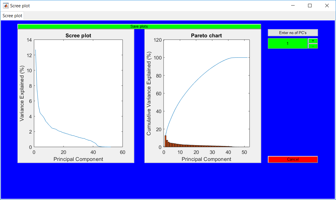
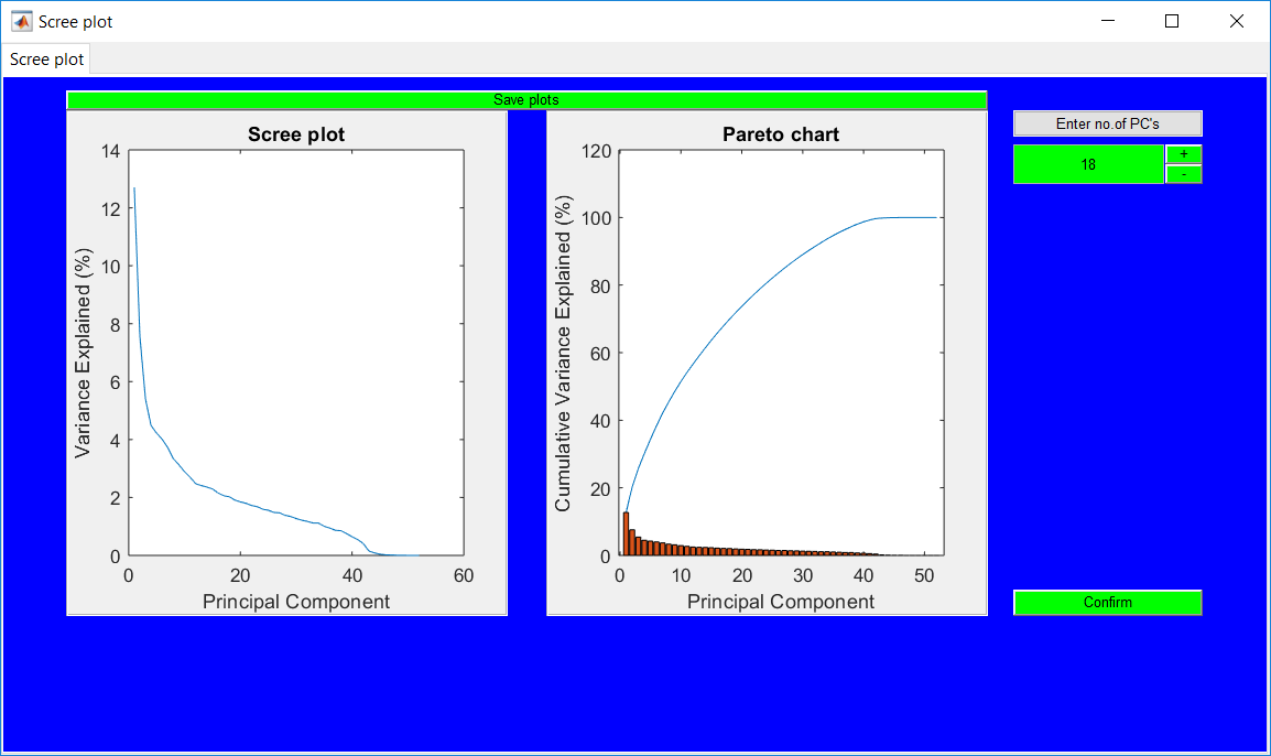
Once the retained principal components are specified for either approach, there is no immediate option to change it. If there is a need to change it, some basic operations can be performed to making the option available again. The first action is to go back by using the ‘Go back’ button before returning to the same page. Another action is to redo the data lag option (if originally ‘No’, just change to ‘Yes’ and change again to ‘No’). The last option is to continue to specify other hyperparameters and view monitoring statistics; an option to update that the retained PCs is provided in there.

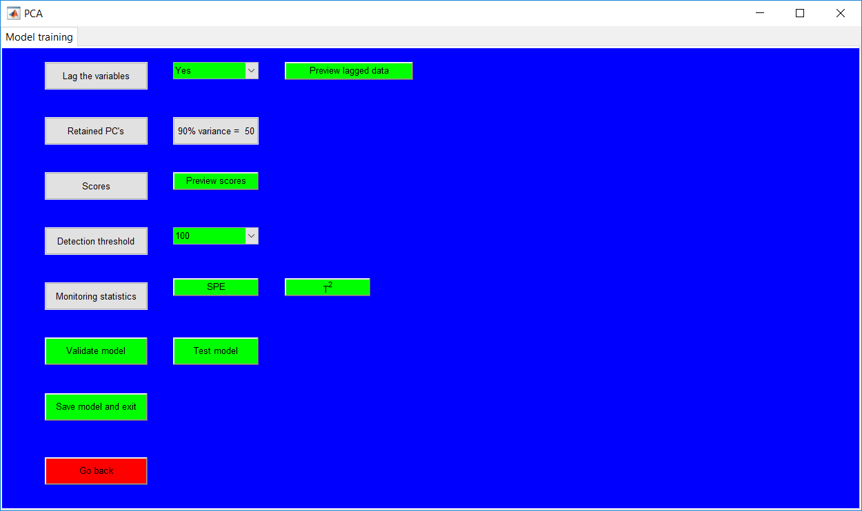
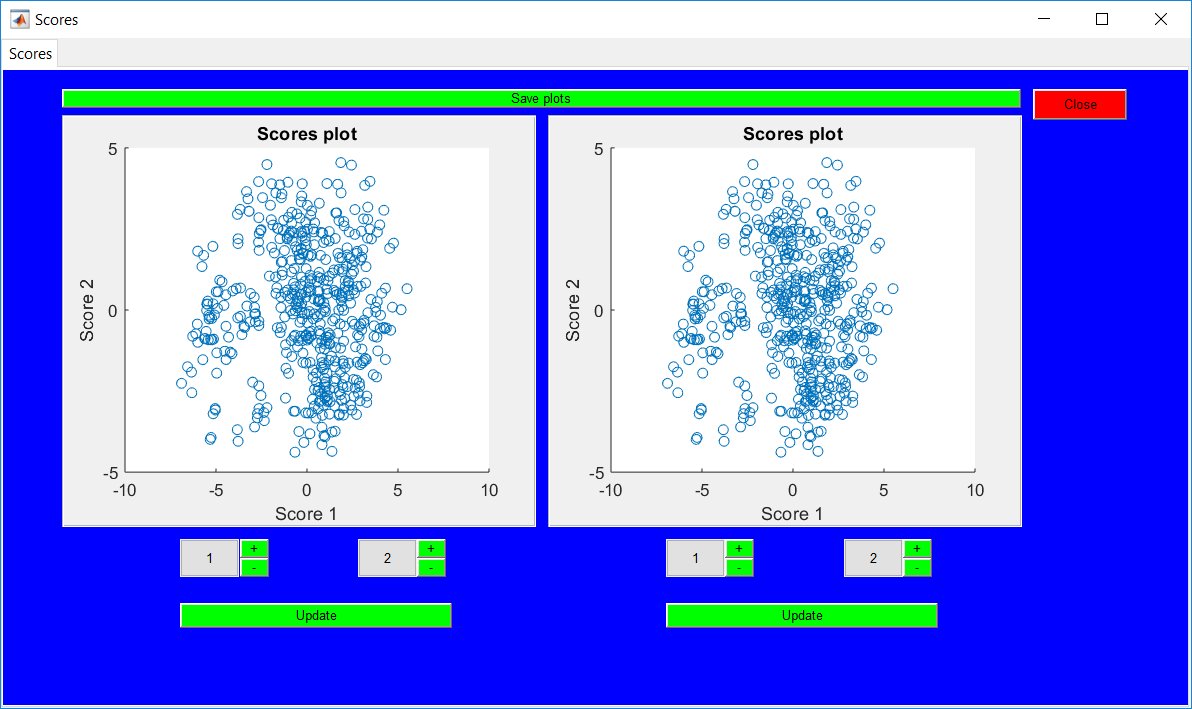
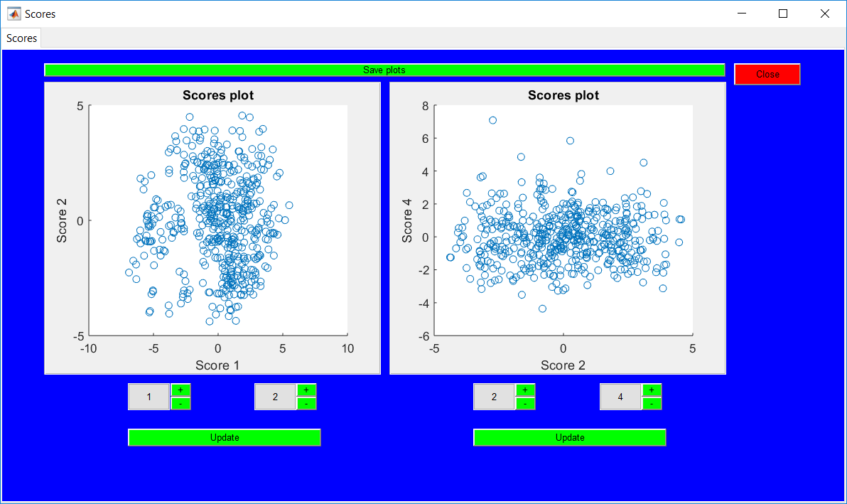
Score plots

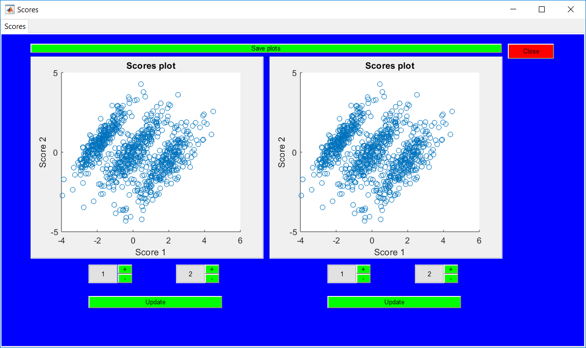
The score plots can be viewed using the provided option. The ‘Scores’ figure created by default presents two subplots for the same scores. The individual charts have buttons to update the score plots.

Detection threshold

The confidence level of the detection threshold needs to be specified by selecting the appropriate value. The selected value just becomes the active value displayed in the drop-down menu.

Monitoring statistics

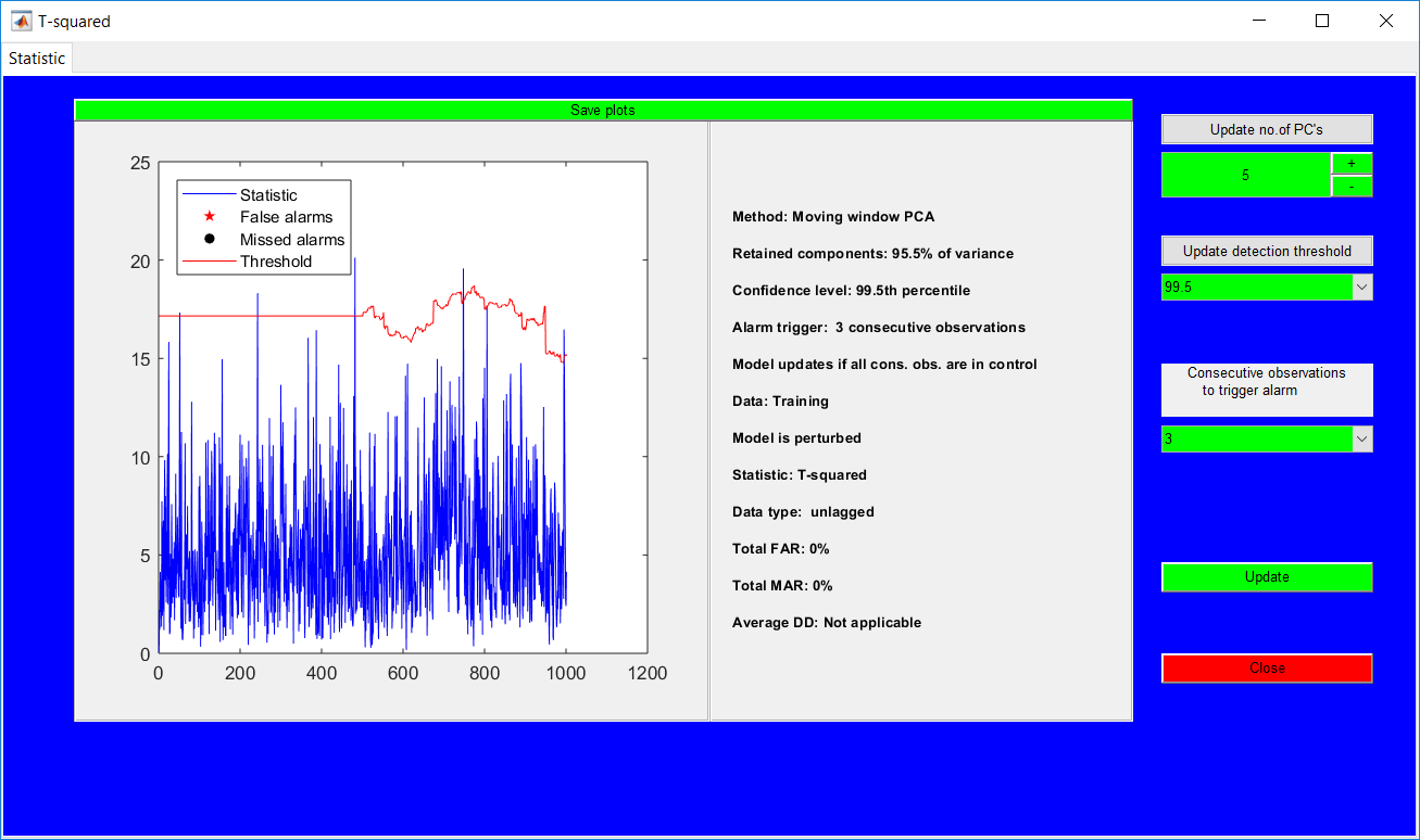
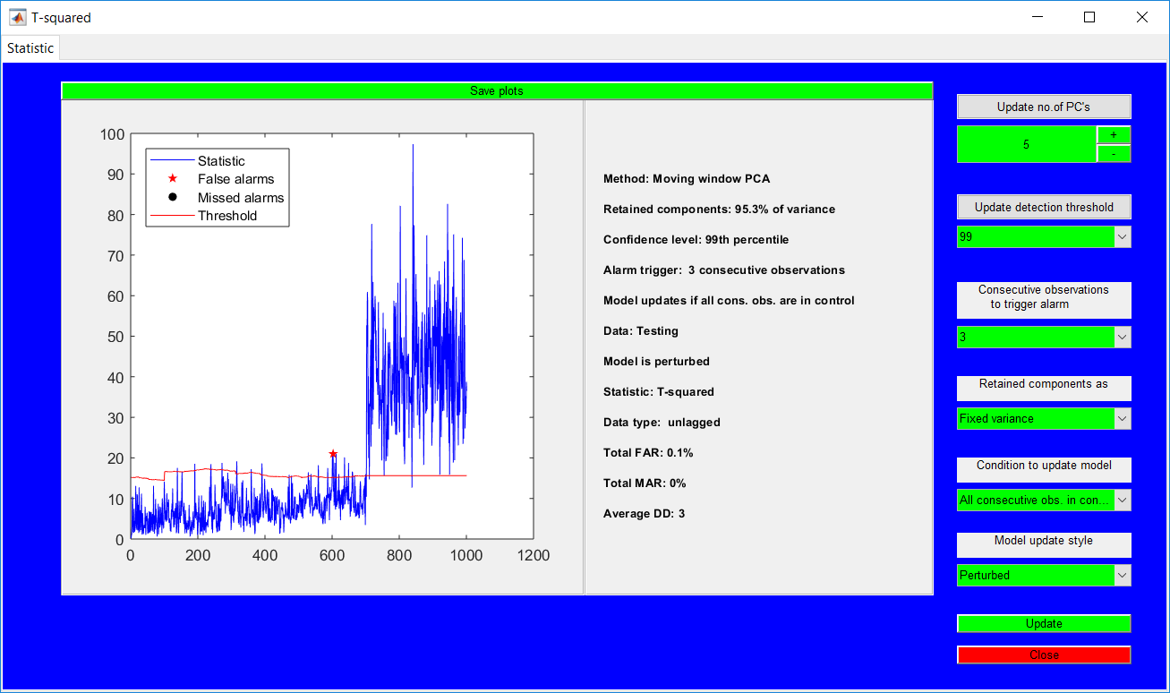
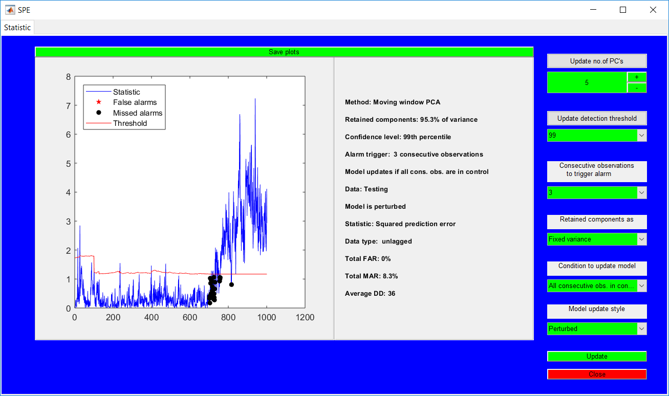
The squared prediction error (SPE) and modified Hotelling’s T² statistics (T²) are provided by their respective buttons. Either button opens the monitoring results figure, with options available for an easier update of the hyperparameters. Also, the summaries are provided for all the inputs specified and the performance metrics. All other entries need to be specified before the monitoring statistics.

The model can be validated, tested or saved afterward. Saving the model automatically creates a model in a specified directory and clears all active figures and workspace. The model can be loaded later.

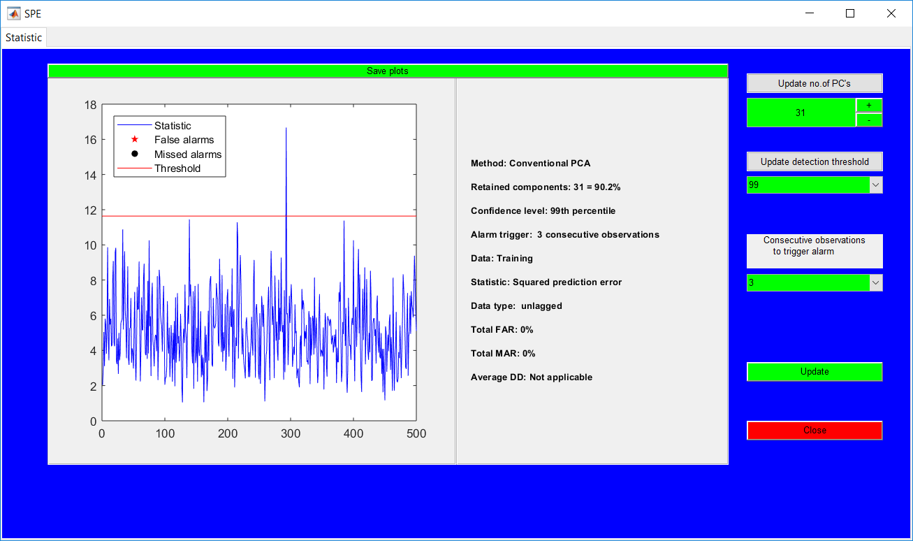
To validate a model, the validation data can be loaded and edited in the same manner as for that for the training. Although there are checks to making sure the trained model and loaded data have a same number of variables, this should be crosschecked to avoid crashes. (The variable increase due to lagged variables is automatically handled). Proceeding from the data selection page leads to the model validation page.

The model validation page provides a summary of the trained model and options to preview the scores, the monitoring statistics, and data if lagged.

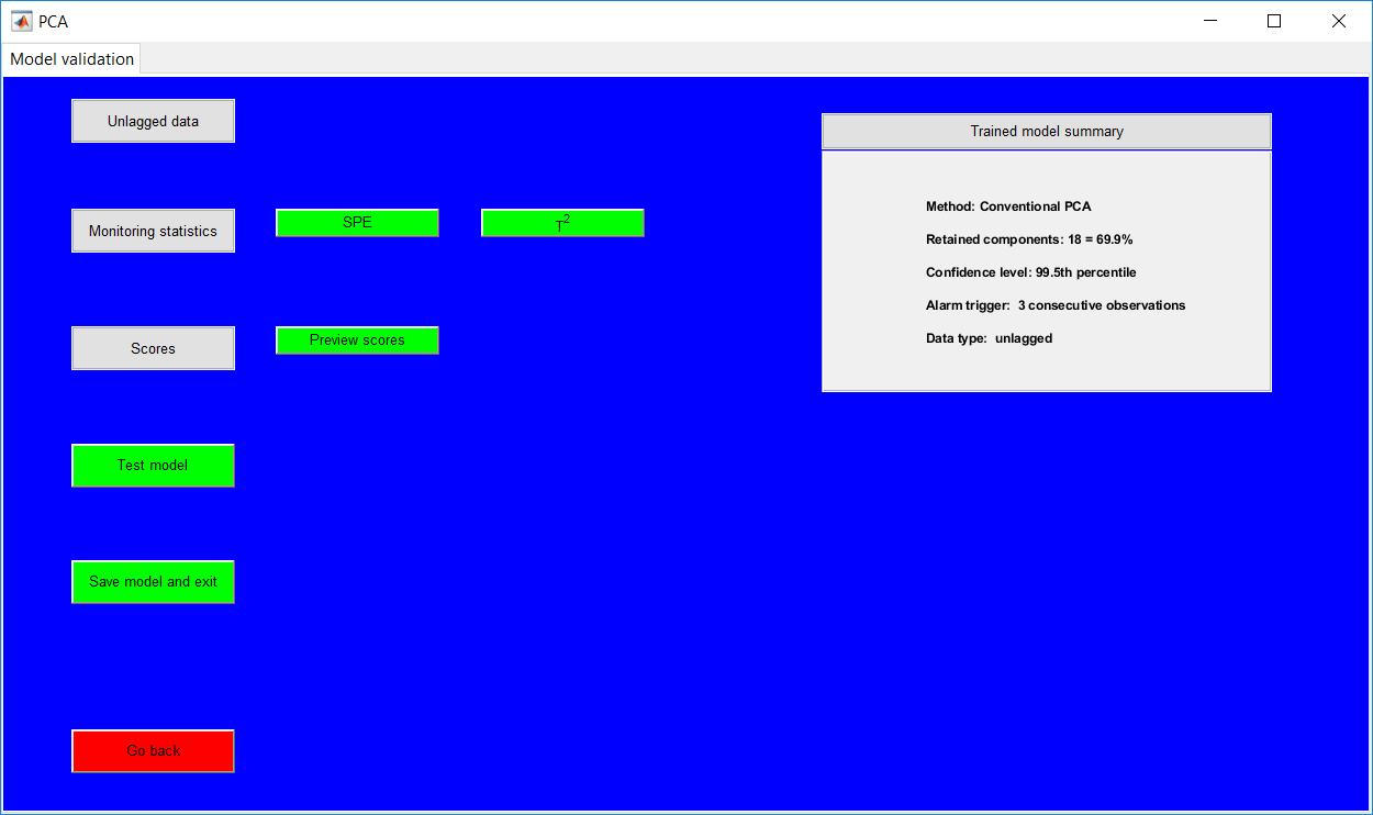
Clicking any monitoring statistics opens the respective results with options to update the trained model hyperparameters. Closing the monitoring statistics provides an additional summary of the current model. If no changes are made, the information presented in the two summaries are the same.

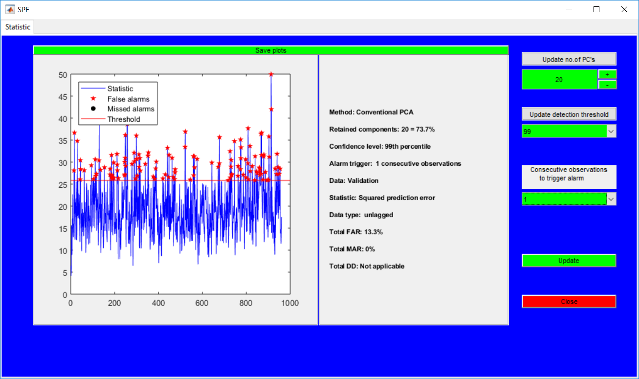
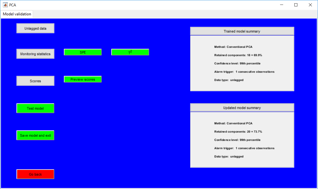
The test model option opens the data selection and an edit option in the same manner as that for the training stage. The additional requirement is the specification of faults in the data.

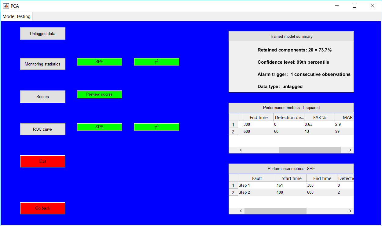
The test page has the same options and appearance as the validation page The additional buttons provided are the receiver operating characteristic (ROC) curves.

Monitoring statistics

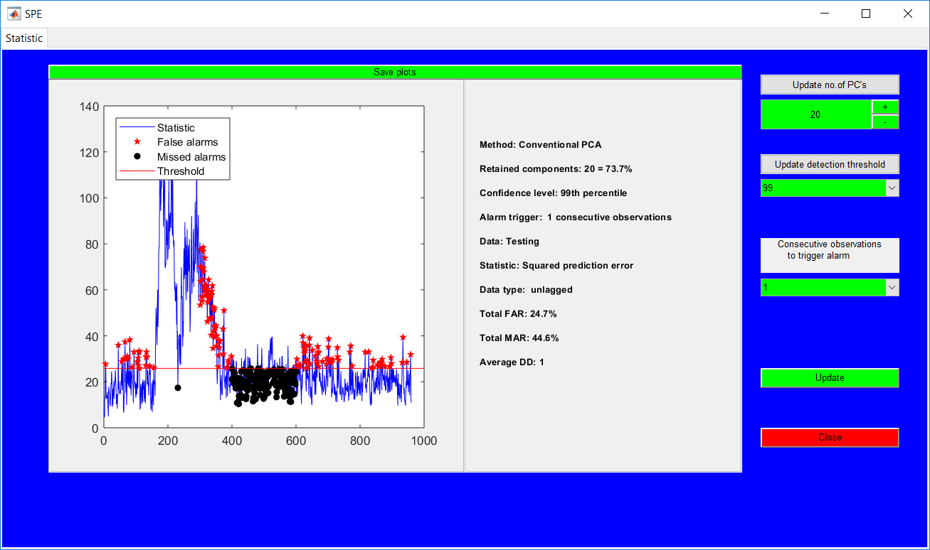
Closing the monitoring statistics figure, however, produces a summary of the performance metrics for the specific faults in a table. Both statistics must be clicked for the results to be displayed. For instance, if the hyperparameters are updated during the SPE preview, the T-squared must also be pre-viewed to provide the updated results as the results displayed are dependent on the active hyperparameters when viewed.

ROC curve

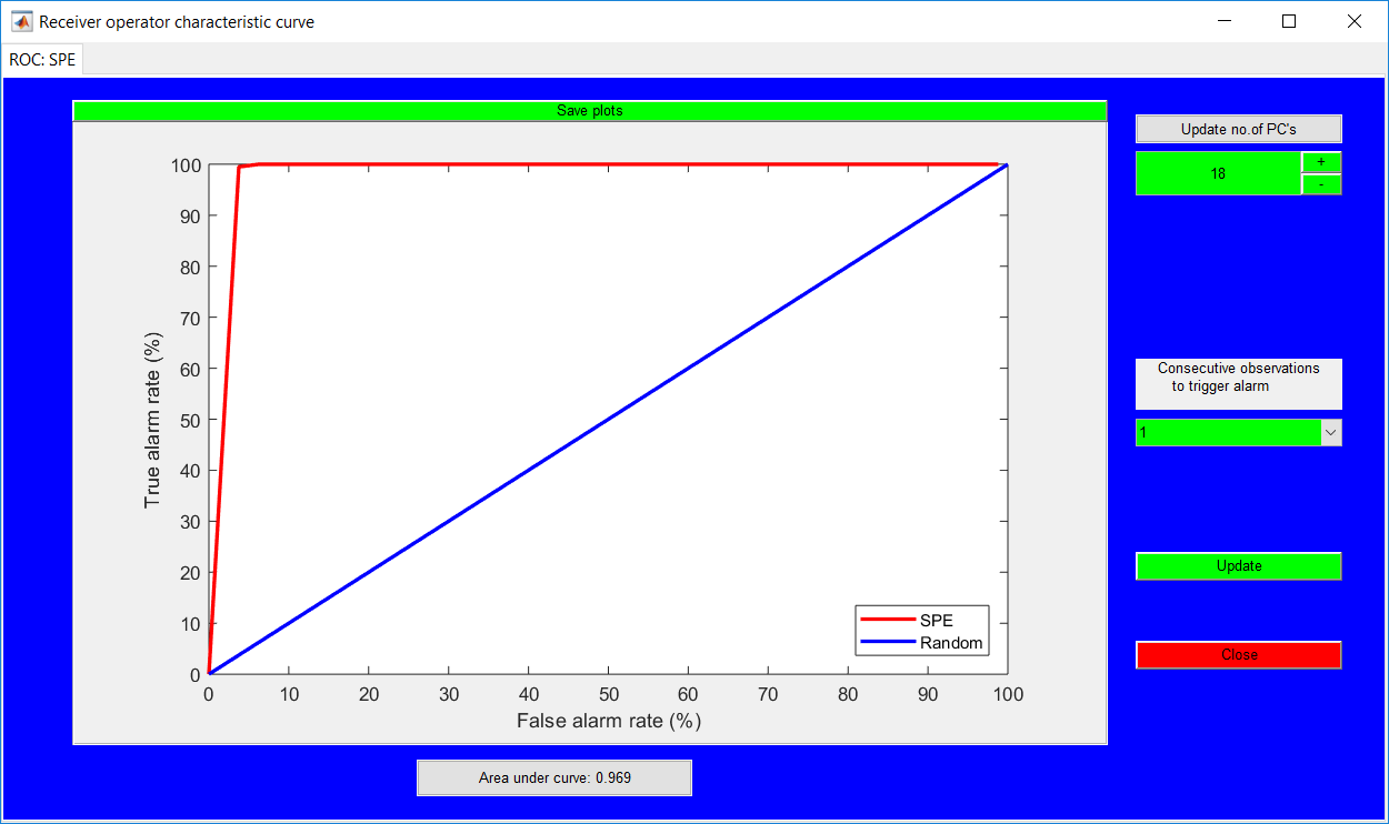
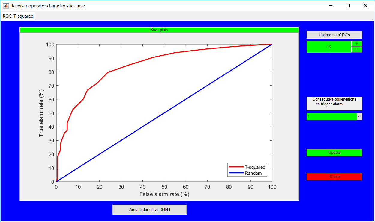
The ROC curve basically provides the monitoring by looking at the effect of different thresholds on the alarm rates. Also, the effect of different retained PCs on the performance as well as consecutive observations required to trigger an alarm can be analyzed by making use of the options provided.

The performance is determined by the area under curve AUC values (expressed in fractions) as shown in the figures. The higher the AUC values, the better.

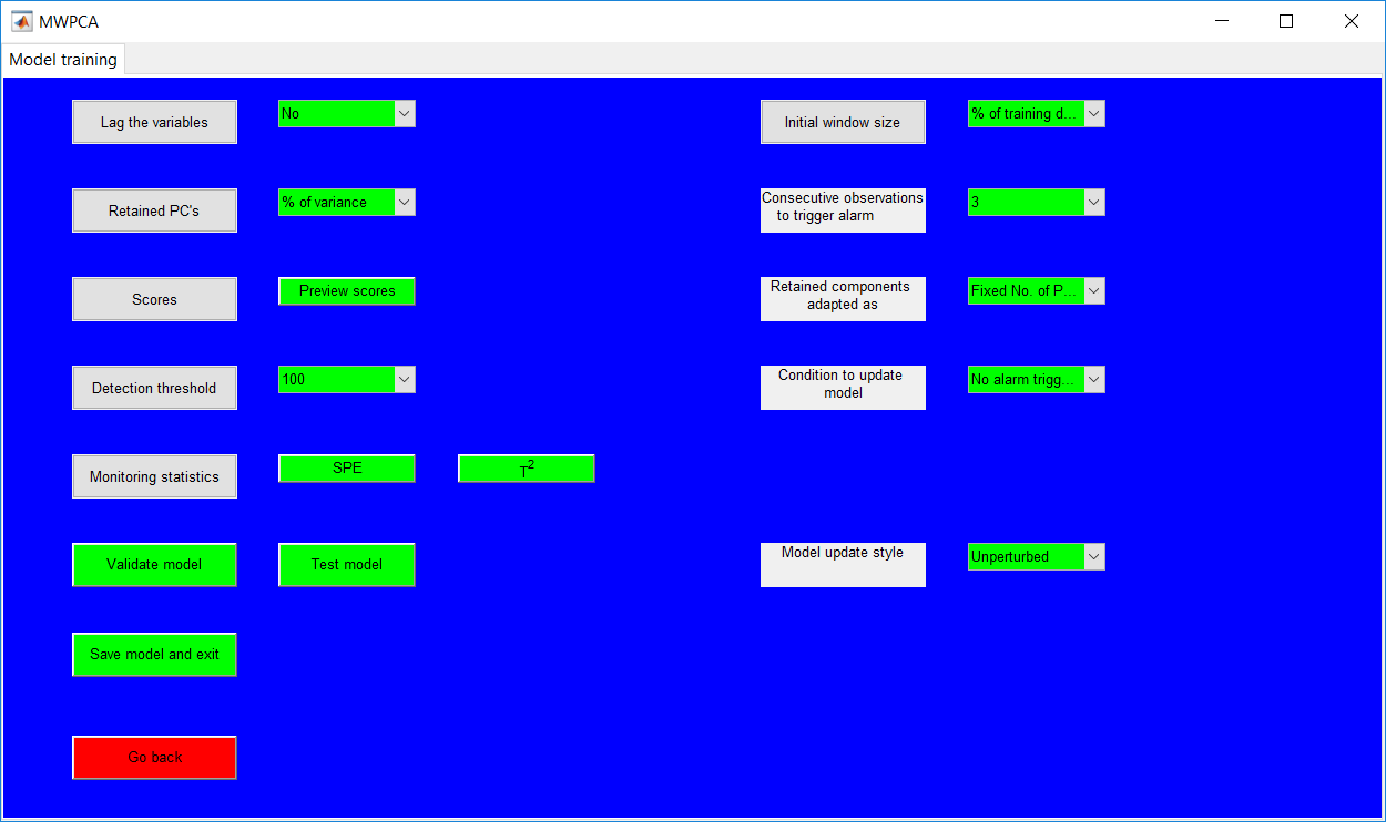
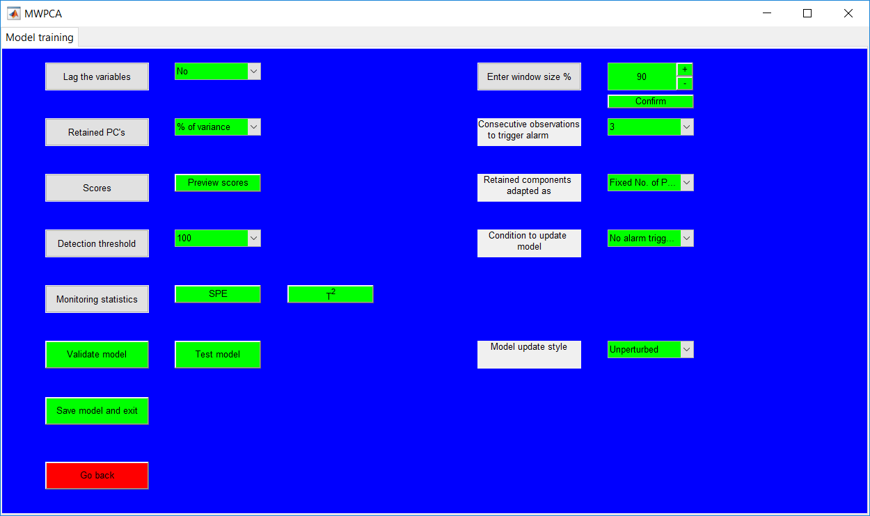
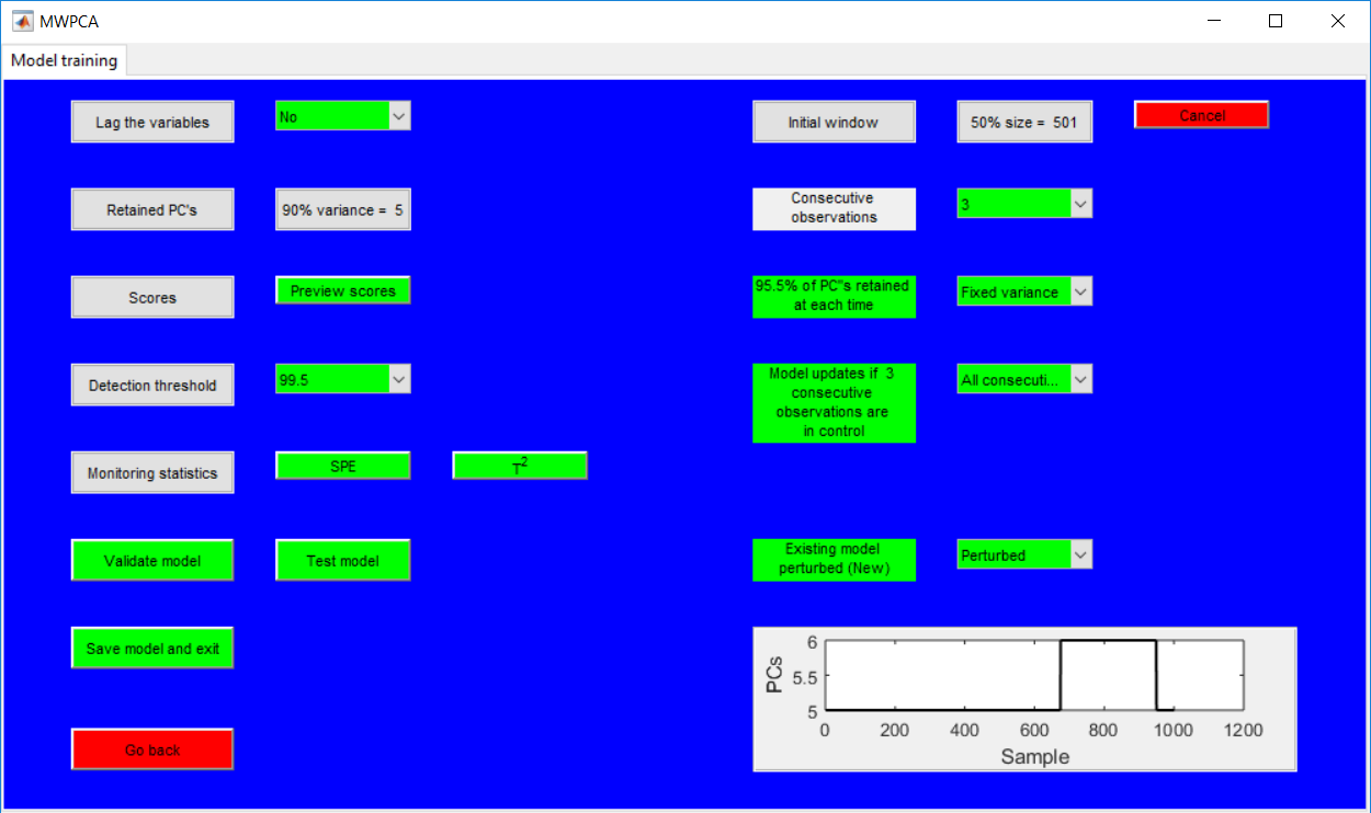
Training page Validation/Test page

In addition to the basic PCA requirements (ordered as left column inputs), the adaptive PCA methods require the inputs in the right column as well. Although the additional inputs required are presented in a column, the overall hyperparameter values must be specified in a row by row approach, i.e. specifying lag the variables, followed by initial window size before retained PCs and then consecutive observations required to trigger an alarm in the manner.

Window size

The initial window size must be entered as a percentage of the uploaded data, if all the data is required, that would be 100%. A basic way to check if the initial window size is accurate is to specify the window size, then retained components and preview the score plots. Basically, a smaller window size would have few observations in the score plots. All of the operations can be undone by just changing the window size again.

Retained PCs adaptation

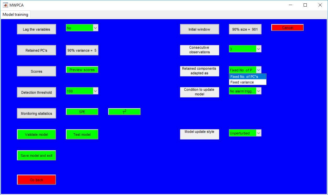
The ‘Retained components adapted as’ requires whether a fixed amount of variance or fixed number of principal components is used at each time stamp. Basically, the same number of principal components may not account for the same variance at each time. It is recommended to you the fixed variance approach.

Model update condition

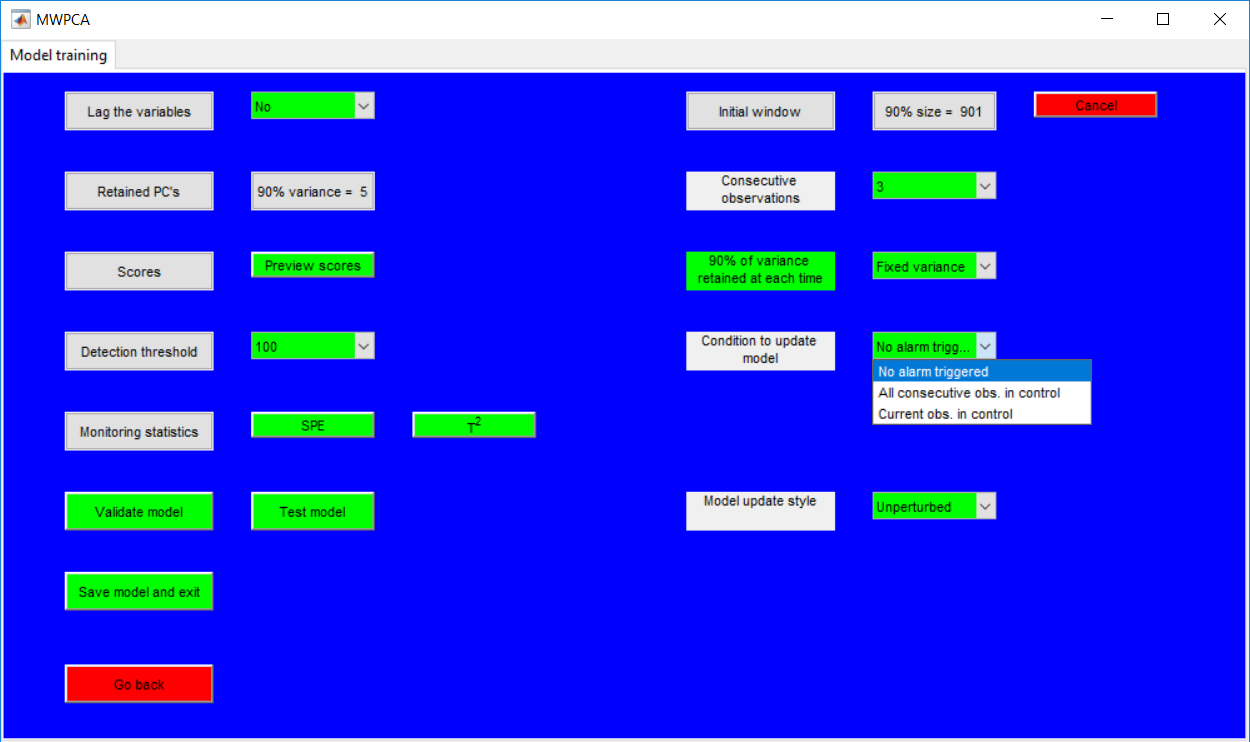
The condition to update model requires the heuristics needed to update the model. The three options provided are: if no alarm is triggered; if the current observation is in control; and if all consecutive observations are in control. If in doubt, use the third approach.

Model update style

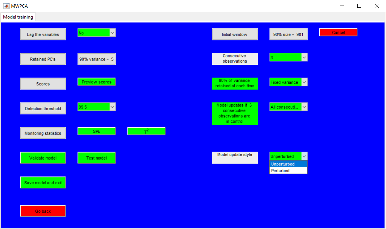
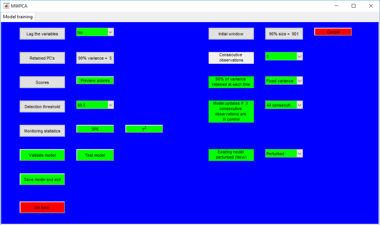
The ‘Model update style’ basically looks at whether the pre-existing model is pseudo-updated (perturbed) or not pseudo-updated (unperturbed). The perturbed option is strongly recommended when the all consecutive observations need to be in control for the model update is used.

Monitoring statistics

The monitoring statistics can be viewed after specifying all the required hyperparameters. Some hyperparameter updates can be easily made from the page.

When the figure is closed, an additional information about the number of retained PCs with time is displayed. For fixed variance, the plot might not be a straight line, as the PCs retained at each time may change.

The validation and test page provide similar options like that for the respective PCA validation/test page. Previewing the monitoring statistics provides extra options to change almost everything selected from the training stage apart from the (initial) window size.

Training page Validation Test page

Information on the lagged variable is similar to that of PCA. Hyperparameter specifications on this page must be done in a row by row manner in order to avoid glitches. The data to be used is specified as well as the level of GMM supervision required needs to be specified.

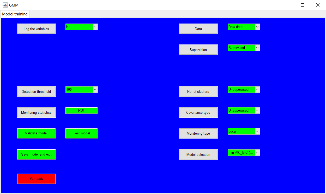
Data type

The Data options provided are the raw data, normalized data (scaled to 0 mean and unit variance), and the PCA scores. Selecting the PCA scores to require the specification for the retained PCs. See information on PCA page with regards to specifying the retained PCs.

Supervision

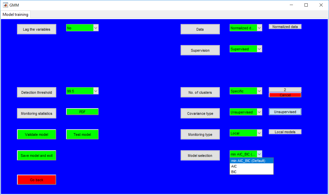
The overall supervision is done by selecting the ‘unsupervised’ or ‘supervised’ approach. In the ‘unsupervised’ case, the extra requirements such as a number of clusters, covariance type, and monitoring approach are automatically not required. What would be needed is the model selection criteria to be employed in determining the best model. The options available are the AIC, BIC, and the minimum AIC-BIC (mAB) criterion. The mAB is recommended.

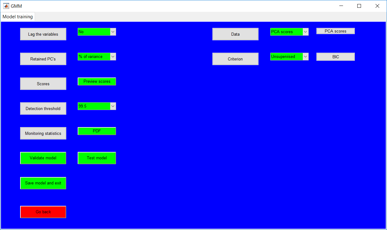
For totally supervised approach, all requirements must be specified by using the provided options. In such a case, the model selection criteria are not used but still need to be specified. A semi-supervised approach can be obtained by keeping the overall supervision as ‘supervised’ but maintaining some of the required hyperparameters as unspecified. In that case, the model selection criteria are key.

Same as PCA, the scores can be previewed for the PCA scores when it is the selected data type. This could be used to just view the scores even if the PCA scores are not the desired data type and then changed afterward.

Monitoring statistic

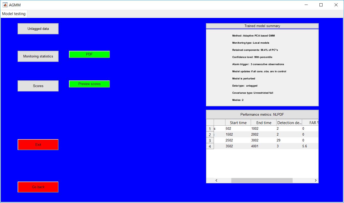
The negative logarithm of the probability density function (NLPDF) is the statistic employed and is activated by using the ‘PDF’ button.

The statistic plots provide options to easily update the hyperparameters and an additional option for the retained scores when the PCA scores are used. Observations belonging to the same mode have the same colour and same threshold. When the monitoring type is changed to global, there is only one threshold (a global one).

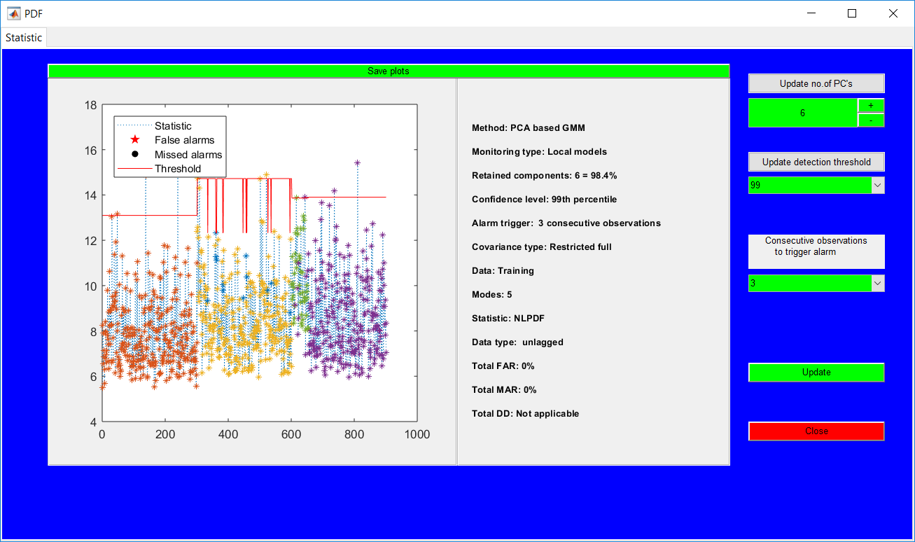
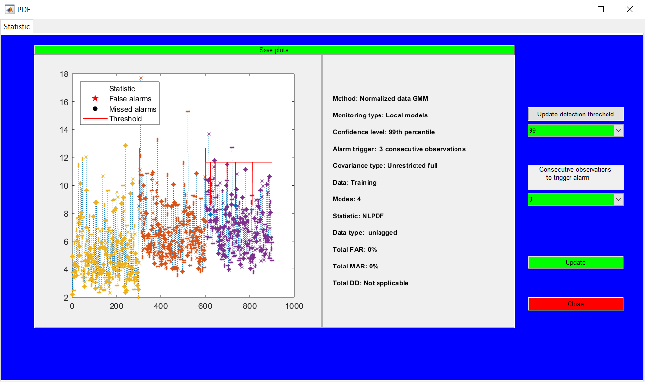
The model validation page is similar to that of PCA which provides a summary of the trained model. The monitoring statistics page, however, opens with extra options than the training stage. The options basically provide the ability to easily change all selected hyperparameters from the training stage.

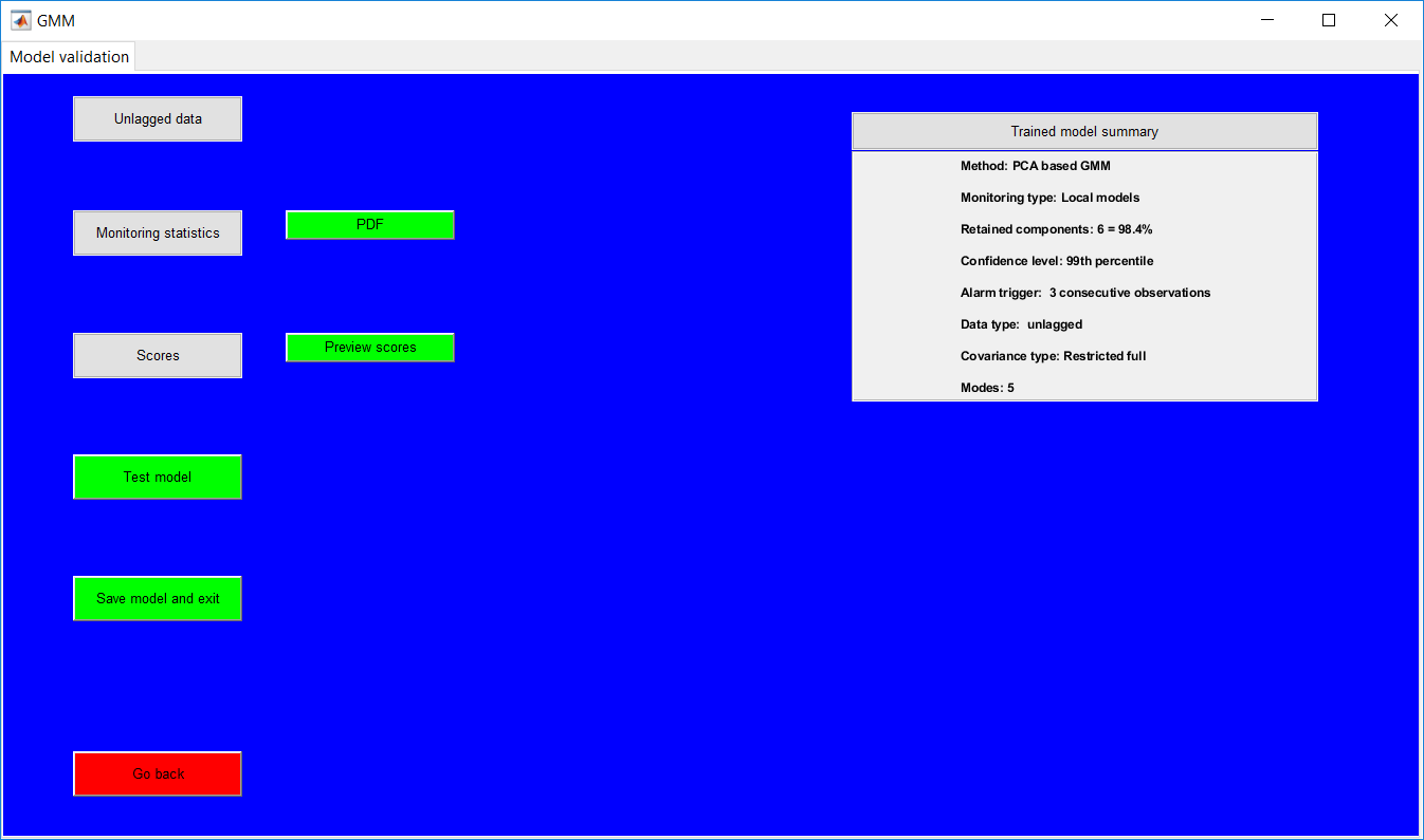
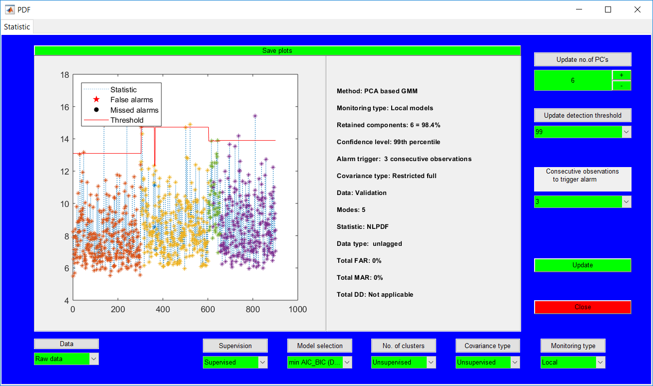
Similar to the PCA validation page, closing the monitoring statistics presents the update summary.

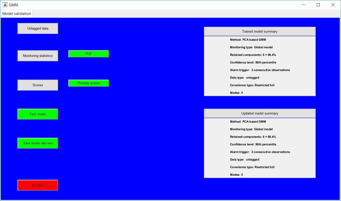
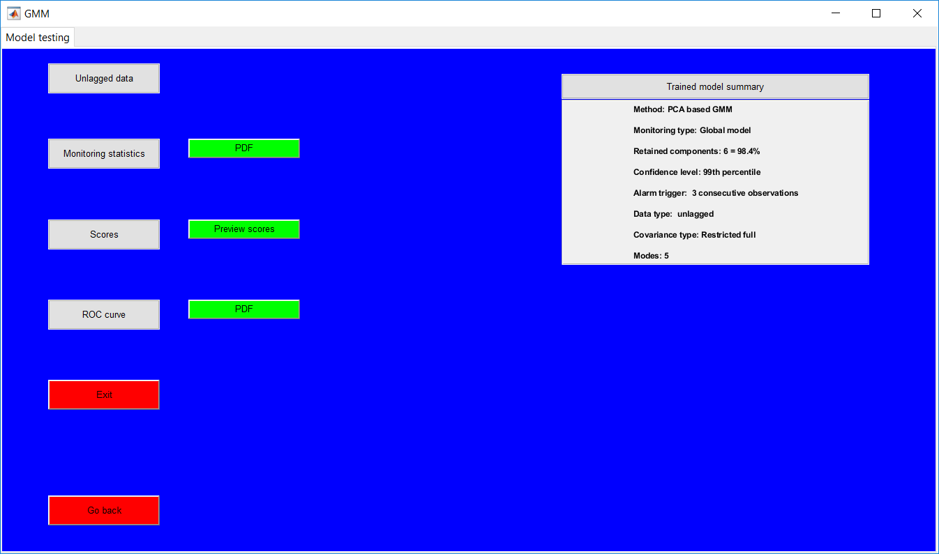
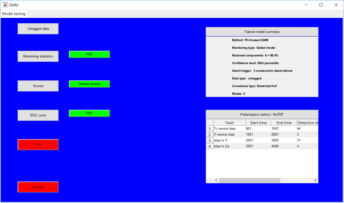
The test page displays similar information as for PCA test page. Opening and closing the ‘PDF’ produces the results summary for the individual faults as presented in the PCA test page.

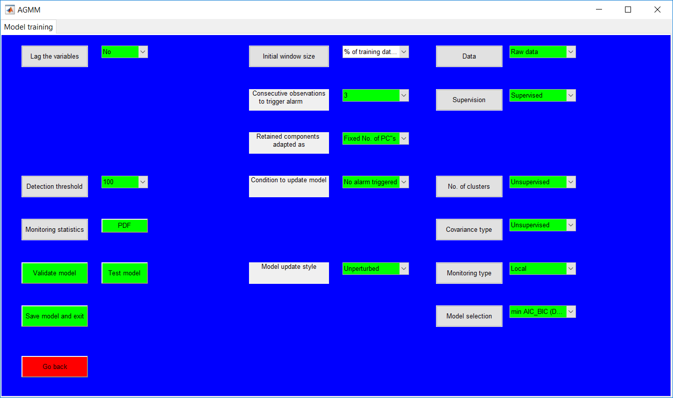
Training page Validation/Test page

The model training page for adaptive GMM presents all requirements from the adaptive PCA and the GMM page. The hyperparameters once more need to be entered in a row by row manner. Instruction on all selections is the same for adaptive PCA and GMM.

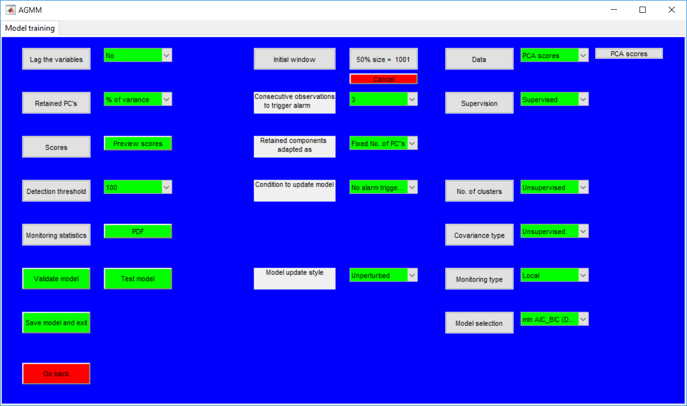
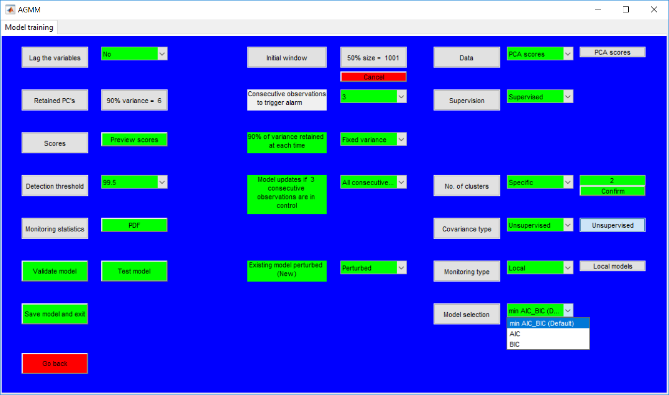
Monitoring statistic

Previewing the monitoring statistics presents periods before the start of adaption having fixed thresholds (there may be jumps when local models are used as each model is monitored by a unique threshold) and variable limits afterward.

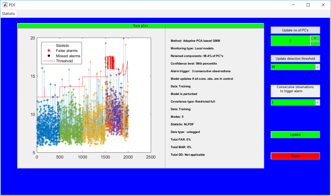
The testing and validation page has a similar outlook as that for the respective PCA validation/test page. Viewing the monitoring statistics, however, provides options to update everything from the training stage apart from the initial window size.

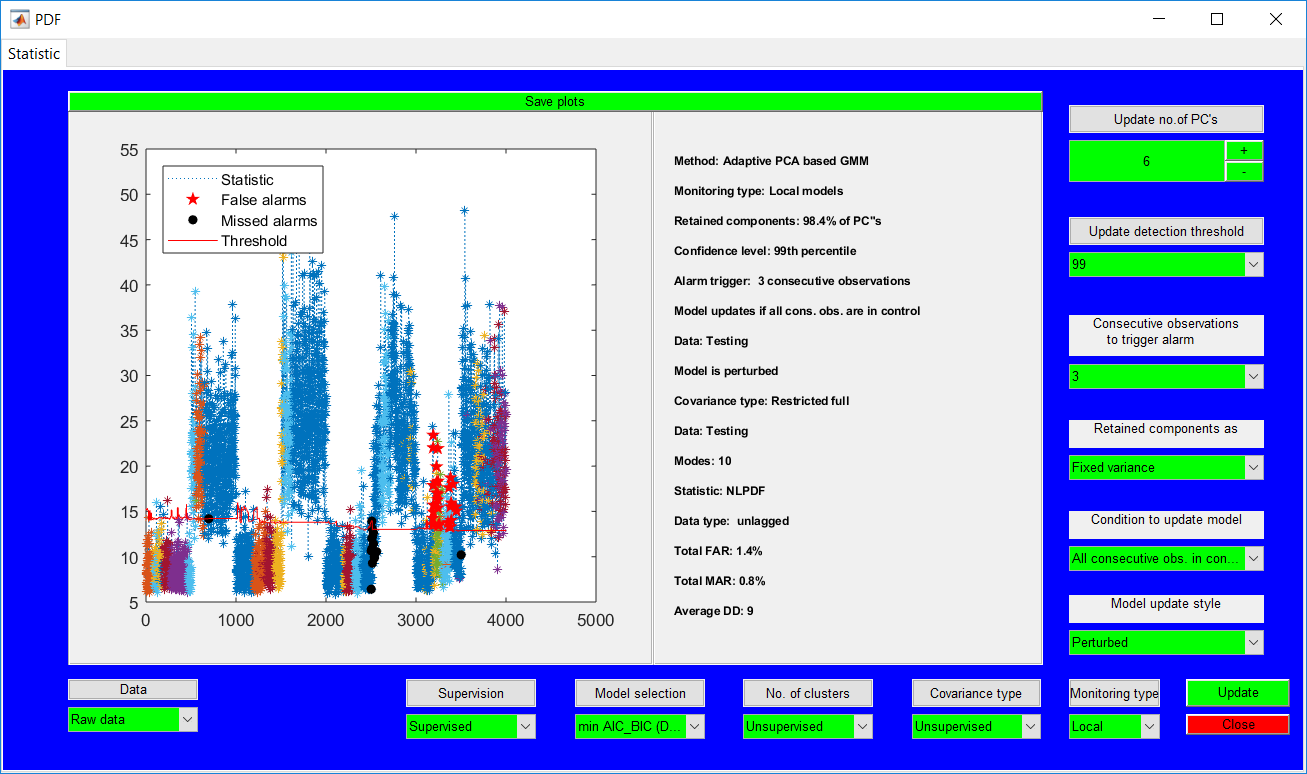
Similar to the other test pages, closing the monitoring presents a summary for the individual faults presents the summary as the others.

MEng Defense, January 2019

Machine Learning Summer School, January 2019

Postgraduate conference, June 2018

Bayesian summer school, January 2018

Mineral research showcase, August 2017

PRINCE ADDO

10811 83 Ave NW, Edmonton, AB| +1-587-99172 | karimprinceaddo@yahoo.com|Personal webpage: princeaddo.cf

RESEARCH INTERESTS

Having a background in the following areas: modelling, machine learning, and graphical user interface with application to monitoring and control of chemical and mining processes; and website, software and application development, Prince seeks to develop further expertise through positions in website and application development, and process improvement and control. Special interests include fault detection and diagnostics, data analytics, graphical user interface development, and full-stack website development.

EDUCATION

PhD, Process Control 09/2020 – Present

Soft sensor development for Alberta oil sands.

University of Alberta, Canada

Master of Engineering, Extractive Metallurgy–Full Research 01/2017 – 03/2019

Thesis title: Adaptive process monitoring using principal component analysis and Gaussian mixture models.

Grade: Pass

Stellenbosch University, South Africa

Bachelor of Science, Petrochemical Engineering 09/2012 – 05/2016

Class: First Class Honours

Class Rank: 1 of 67

Kwame Nkrumah University of Science and Technology (KNUST), Ghana

CONFERENCE PUBLICATION

Addo P., Auret L., Kroon S., & McCoy J.T. (2018, October). Adaptive process monitoring using principal component analysis and Gaussian mixture models. Presentation at the Control Systems Day of the South African Council for Automation and Control, Stellenbosch, SA.

Addo P., Wakefield B., Auret L., Kroon S., & McCoy J.T. (2017, August). Adaptive process monitoring using principal component analysis, a milling circuit focus. Presentation and poster presented at the Minerals Research Showcase of the Southern African Institute of Mining and Metallurgy, Cape Town, SA.

AWARDS

University of Alberta Doctoral Recruitment Scholarship, ($15,000 per annum) 2020 – Present
The Centre for Artificial Intelligence Research (CAIR) bursary, CAIR-South Africa (R90,000 per annum) 2017 – 2018
Best student award, College of Engineering, KNUST (College Awards) 2012 – 2016
Ing. Dr Adu Amankwah award for the best graduating student, Dept. of Chemical Engineering, KNUST 2016

ACHIEVEMENTS

Founder and lead developer for Ghanaian website and software development start-up company – Ultimate Developers (https://ultimatedevelopers.digital/).
Developed a non-isothermal continuous stirred tank reactor simulator which is available for open access (see https://prince-addo.github.io/).
Developed a process monitoring toolbox which is available for open access (see https://prince-addo.github.io/).

RESEARCH EXPERIENCE

Academic

Masters work 01/2017 – 03/2019

Adaptive process monitoring using principal component analysis and Gaussian mixture models.

Worked on improving process monitoring performance in process industries (mainly chemical and mining), by developing process monitoring models which incorporate process changes and update the model parameters in real time.

Undergraduate Honours Research Thesis 09/2015 – 05/2016

Plant design for styrene production

Served as a project leader in the design of a plant to produce styrene in Ghana, carrying out the required feasibility studies, economic and environmental impact assessments. The final thesis was assessed in through a thesis defence.

Engineering in Society Project 05/2013 – 09/2013

Pyrolysis of plastic waste into fuel oil

Investigated the feasibility of converting locally produced plastic waste (generated in communities) into a mixture of synthetic crude oil. The result of this study was used in the development of a pilot programme for a first-year project to help students identify the application of engineering to everyday challenges– and was presented to the College of Engineering, KNUST.

Industrial

Chemical Engineer Intern, Genser Energy, Ghana. 06/2014 – 08/2014

Projects undertaken:

Assessment of binders for coal briquettes

Investigated the performance of local binders for the production of coal briquettes in power production for GP Chirano Plant, a 30.0MW Steam Turbine Plant.

Assessment of biomass for coal co-firing

Investigated the performance of different biomasses to be combined with coal for power production.

WORK EXPERIENCE

Genser Energy, Accra, Ghana private power producer in Africa

Chemical engineer intern: 6/2014 – 8/2014

Treated coal and installed new machinery at the storage facility.
Researched on suitable binders for coal briquettes.
Researched on suitable renewable resources for co-firing in a gasification plant to produce power.

PROGRAMMING SKILLS

MATLAB

PHP

Python

JavaScript

Prince Addo

Prince Addo

Chemical and Materials Eng Dept
University of Alberta
Edmonton AB

Dr. Lidia Auret

Dr. Steve Kroon

Dr. Roelof Coetzer

Dr. John McCoy

MEng Defense, January 2019

Machine Learning Summer School, January 2019

Postgraduate conference, June 2018

Bayesian summer school, January 2018

Mineral research showcase, August 2017

Miscellaneous

EDUCATION

PhD, Process Control 09/2020 – Present

Master of Engineering, Extractive Metallurgy–Full Research 01/2017 – 03/2019

RESEARCH EXPERIENCE

Academic

Industrial

Follow me on social media

Facebook

LinkedIn

Github

Copyright © 2018-2021 Prince Addo. All rights reserved.

Prince Addo

Prince Addo

Chemical and Materials Eng DeptUniversity of AlbertaEdmonton AB

Dr. Lidia Auret

Dr. Steve Kroon

Dr. Roelof Coetzer

Dr. John McCoy

MEng Defense, January 2019

Machine Learning Summer School, January 2019

Postgraduate conference, June 2018

Bayesian summer school, January 2018

Mineral research showcase, August 2017

Miscellaneous

EDUCATION

PhD, Process Control 09/2020 – Present

Master of Engineering, Extractive Metallurgy–Full Research 01/2017 – 03/2019

RESEARCH EXPERIENCE

Academic

Industrial

Facebook

LinkedIn

Github

Copyright © 2018-2021 Prince Addo. All rights reserved.

Chemical and Materials Eng Dept
University of Alberta
Edmonton AB